
What exactly is Denoising Score Matching?
What is Denoising Score Matching? Why is it central to Diffusion Models?

In the previous article, we had looked at the technique of score matching where the objective was to match the predicted score function with the true score function.
Here is the link to the article:

We encountered a challenge where we thought that since we do not know the true score function, how can we ever match our predicted score with it?
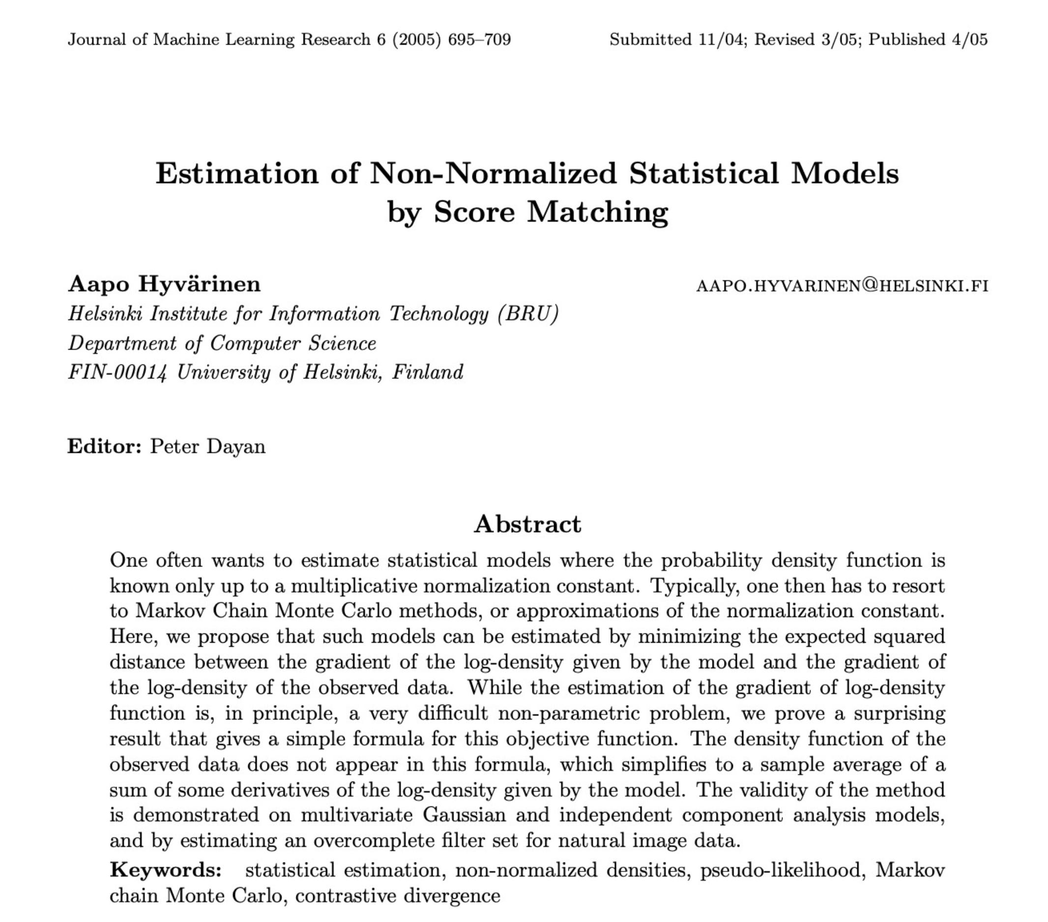
This paper came to the rescue where we found an alternative loss function that only requires the data samples.
This loss function looked as follows:
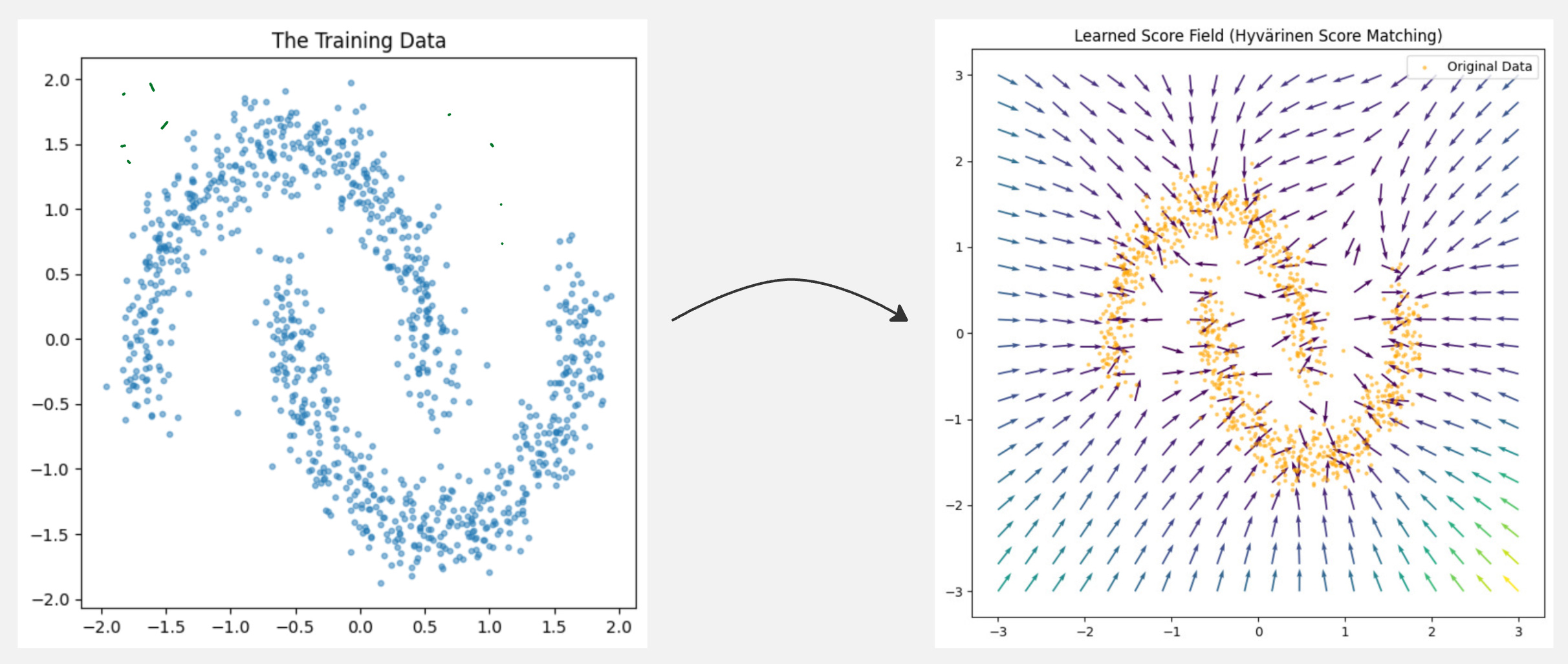
We looked at an example where, for a given set of data samples, we learned to find a score function using the above formulation.
This is excellent, but this technique is not used in practice. Let us understand why.
To calculate the trace of a matrix of dimension D, we need to calculate all the elements of the matrix which are D x D.
The order of complexity scales as the square of the dimension of the matrix. This becomes extremely computationally expensive for larger matrices.
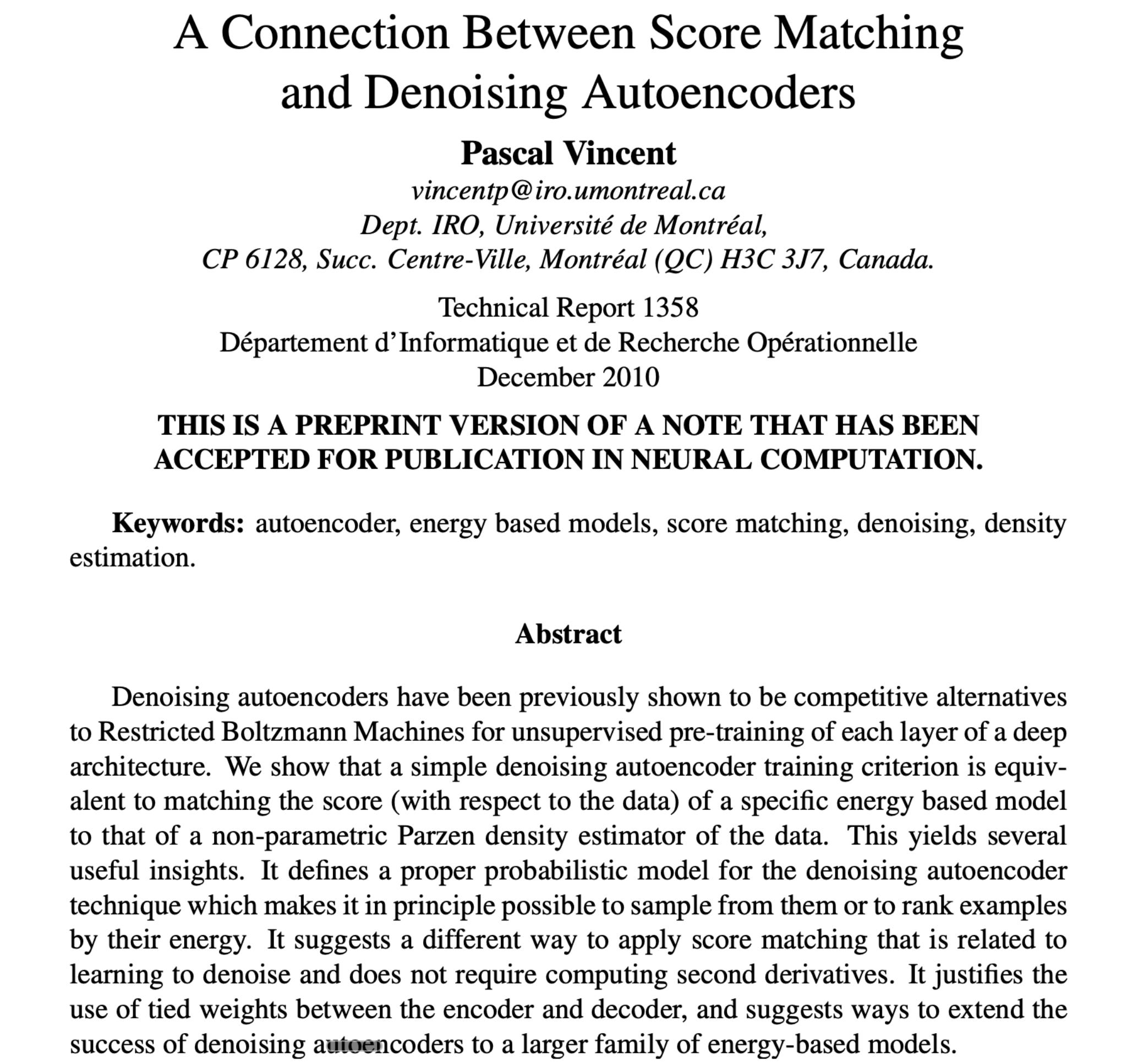
This technique was introduced by Pascal Vincent in 2010.
What Pascal Vincent said was very interesting. To understand what he said, let us take a practical example:
Imagine you have a tabletop. There are invisible magnets hidden at specific spots on this table. These magnets represent your Real Data.
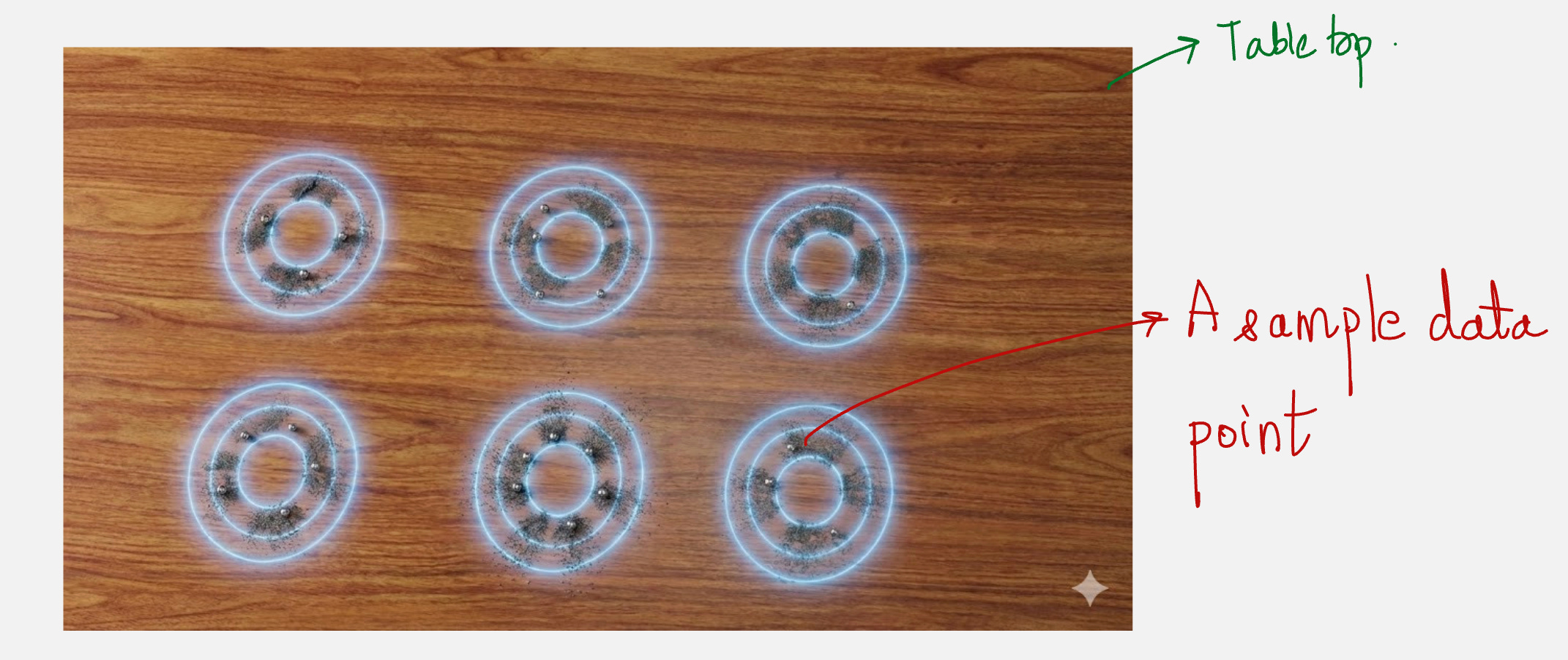
Your goal is to draw a map of the magnetic field that tells you, for any point on the table, which direction the nearest magnet is pulling.
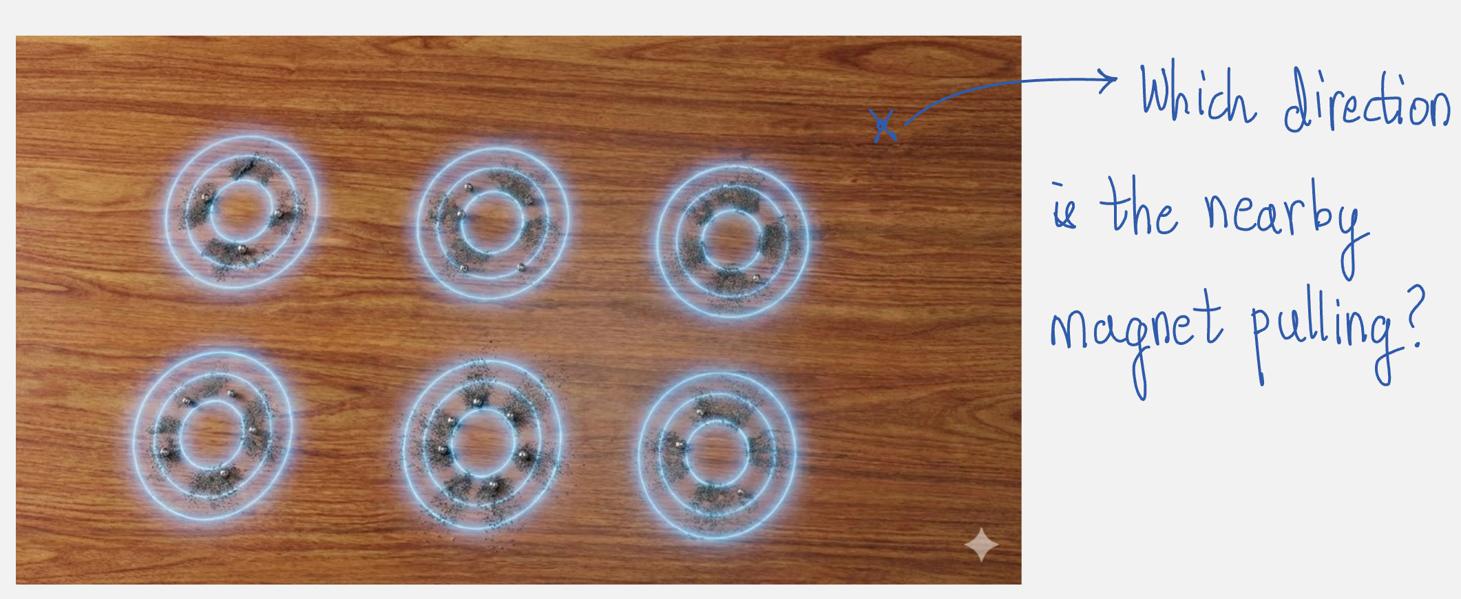
If you just look at the empty table, you can’t calculate the magnetic field. You don’t know where the magnets are or how strong they are. For example, there might be more magnets than you see and you do not know the magnetic field at all places.
Okay, now we do a small trick:
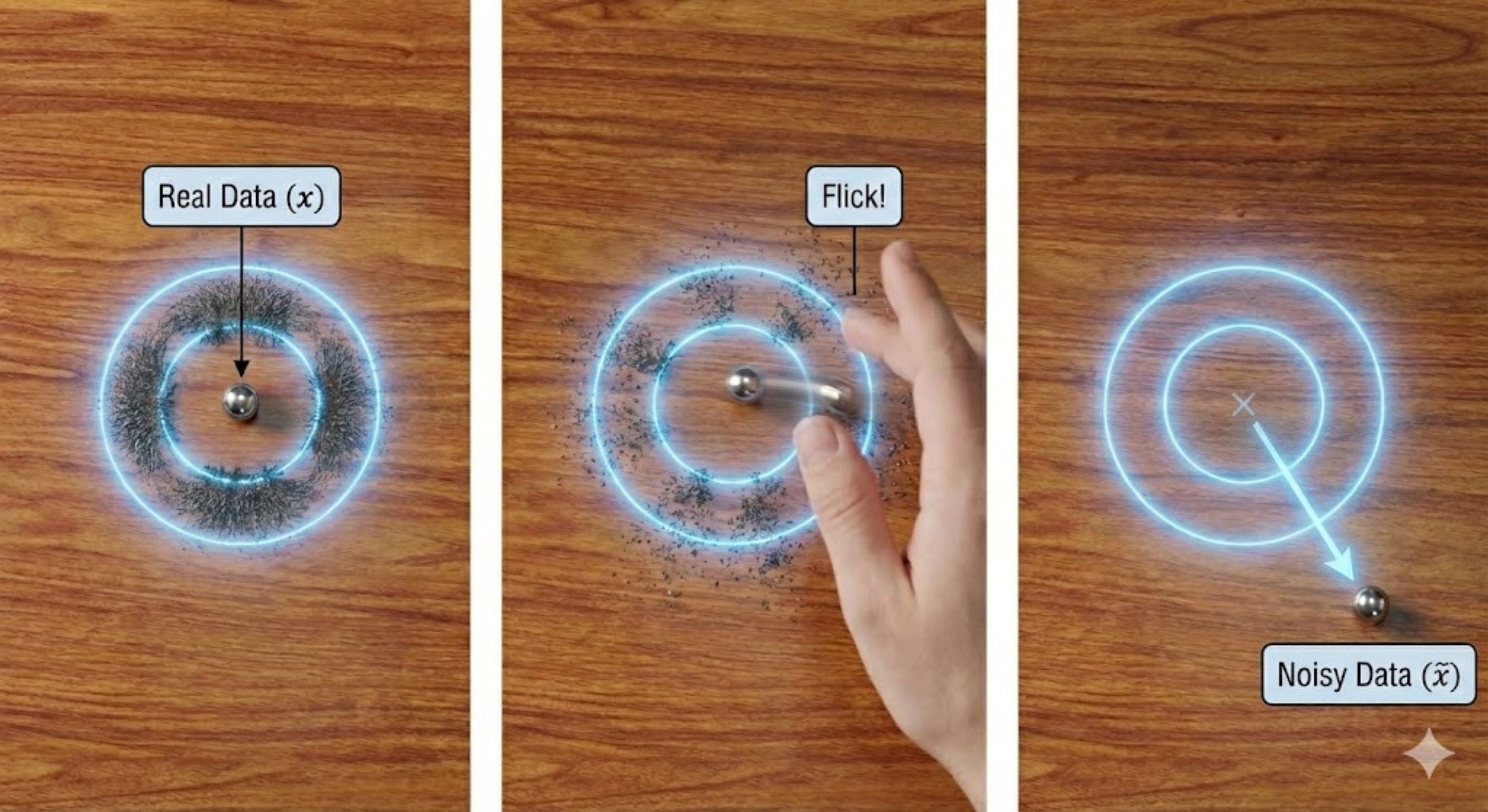
We place a metal ball exactly on top of a hidden magnet. We flick the ball in a random direction. It rolls away and stops at a new, random spot. This is the Noisy Data.
Next, we bring in a student:
We show the student the ball’s new location
We hide the original magnet location
We ask the student, “Draw an arrow representing the force needed to pull this ball back to where it started.”
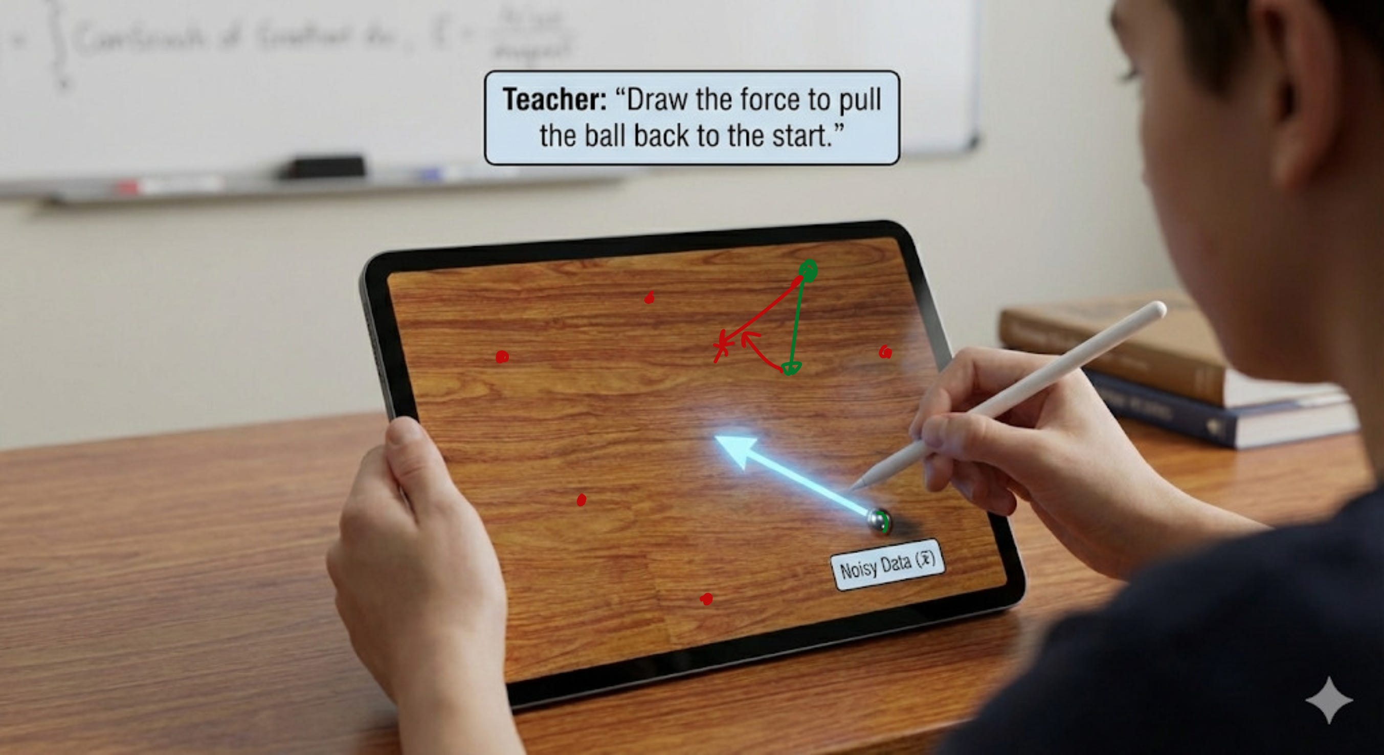
The student has no idea where this noisy data came from.
But we know where it came from.
So if we can give the student feedback based on the student’s prediction and our knowledge, we can teach the student how to draw the force to pull the ball back to the starting point for every possible noisy data in the field.
So through this process, wouldn’t the student learn the magnetic field at all points in the field?
Now, let us look at how this analogy relates to Vincent’s ideas in his paper.
The hidden magnets in the analogy represent the real, clean data points. This is denoted by the following symbol:
The “flick” represents noise added to the clean data points. The noisy data (ball’s new spot) is represented as follows:
The probability distribution of the noisy data is represented as follows:
Here, sigma represents the noise added to the data.
The student represents the neural network trying to guess the direction back to the magnet. This is represented as follows:
The correct arrow from the original data to the noisy data denotes the score function for the distribution of noisy data, it is denoted as follows:
Hence the loss function boils down to the following:
The conditioning technique (probability of the noisy data, given the original data) also appears in the variational view of diffusion models in DDPM.
We can actually simplify this further to get a very simple loss formulation:
If we assume that the noise is Gaussian, we can simplify the score function, which we want to learn.
If we add a Gaussian noise with variance σ^2 to each data point, then we can write the following:
Let us consider the Batman example, which we have looked at in some of the previous articles as well:
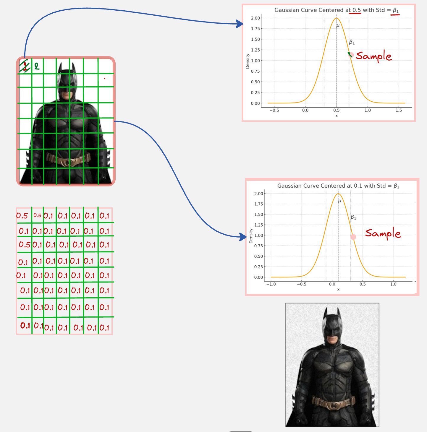
In this image, what we have done is we have taken a pixel from the Batman image and then added noise to that pixel. The addition of noise is done by sampling using a Gaussian distribution with the same mean as the pixel value and the standard deviation as the noise level.
We do a sequence of mathematical steps below to calculate the target for our loss function (it is not complicated, trust me!)
First, we write down the probability distribution for noisy sample, given the original sample as follows:
This formula comes from the Gaussian distribution formula.
Now, if we take the logarithm of the above and then take the derivative, we get the following:
Hence the Denoising Score Matching loss simplifies to:
This objective function tells you that you are training your score function to predict the noise which is added to create the noisy distribution.
In the context of our previous example, this means that you are trying to guess the direction of the flick.
Doesn’t this remind you of Denoising Diffusion Probabilistic Models (DDPM) where we came to the same conclusion towards the end? [Refer to this article written by us:

Let us take a practical example to understand how this is implemented:
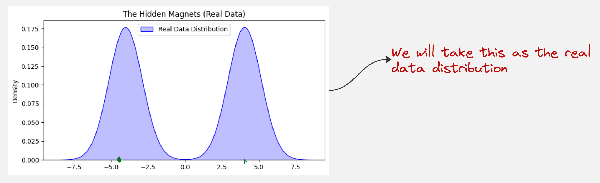
We will be using the method of Denoising Score Matching to predict the score function for this data distribution:
Here is the link to the Google Colab notebook which is used for this practical:
Google Colab Notebook for Denoising Score Matching
This is how our learned score function behaves after the training is completed:
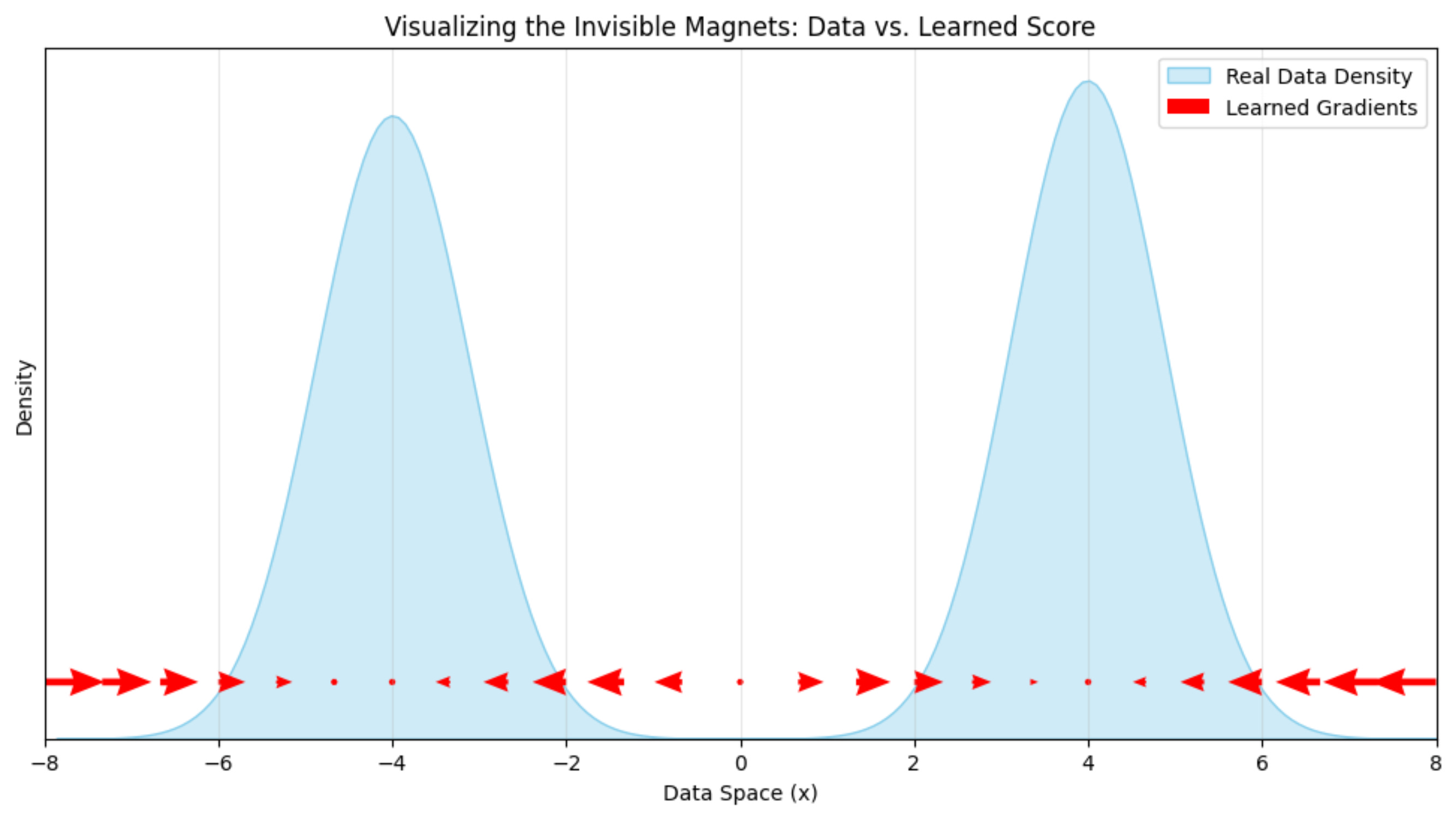
This looks correct because the arrows are pointing towards the direction of the data.
You might have guessed what we are about to do next.
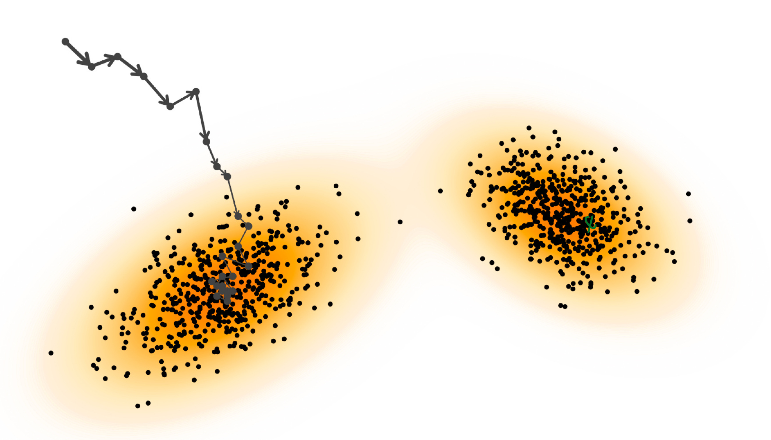
Once the score function is learned, let us sample from it using Langevin Dynamics.
We have already seen the formula for this, which looks as follows:
This is our “drunker hiker” who is taking steps to move towards the data samples. See the image below:
On applying Langevin Dynamics to the above example, this is what we get:
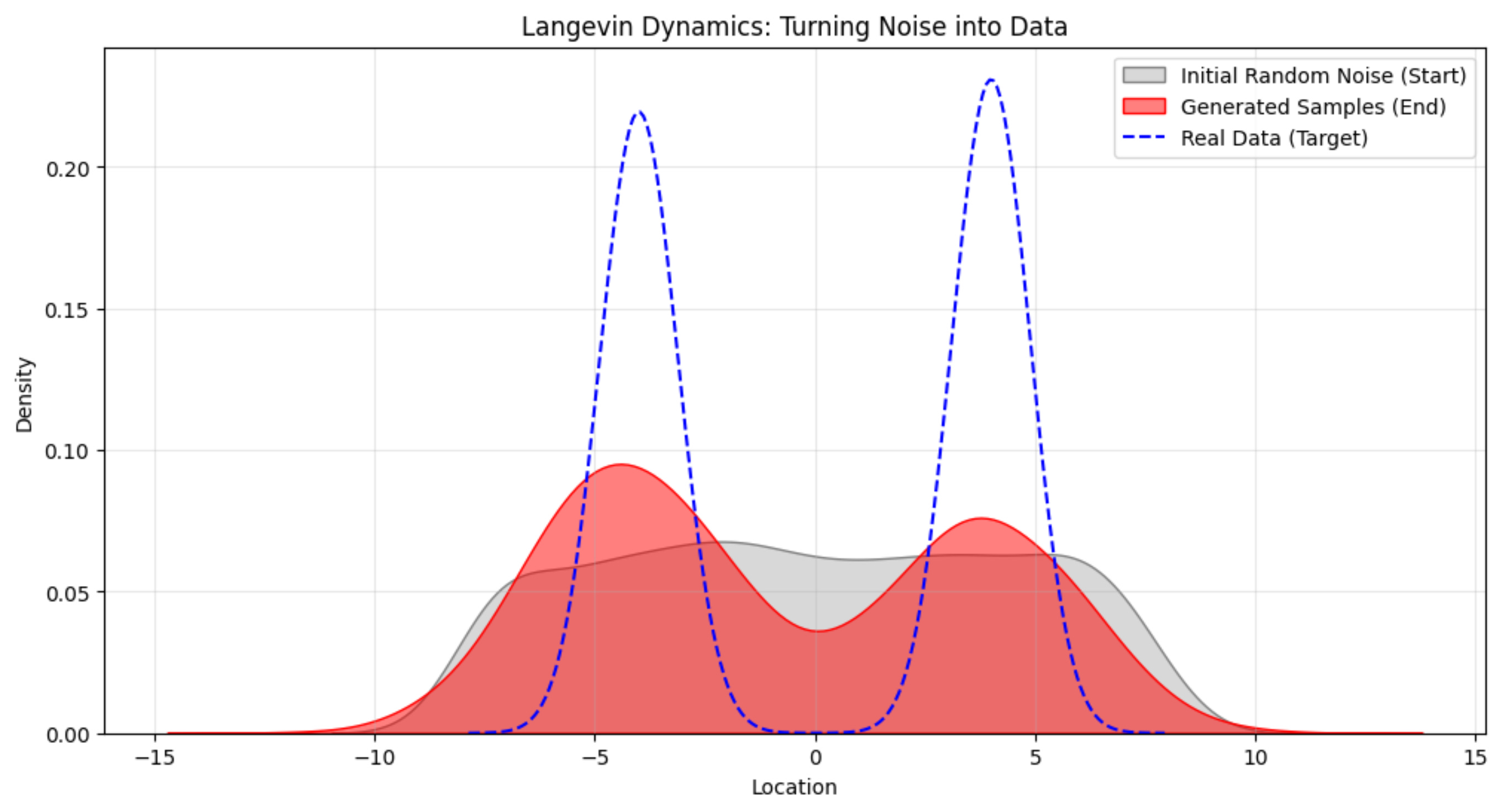
The generated distribution does not match the true distribution perfectly with the density, but you can see the two peaks located at the same location as that of the true data distribution, which is exactly what we want.
That’s it!
Here is the link to the original paper which introduced DSM (Denoising Score Matching): https://www.iro.umontreal.ca/~vincentp/Publications/smdae_techreport.pdf
For more detailed proofs, please refer to the book: The Principles of Diffusion Models From Origins to Advances (https://arxiv.org/abs/2510.21890) [Pages 68-79]
If you like this content, please check out our bootcamps on the following topics:
Modern Robot Learning: https://robotlearningbootcamp.vizuara.ai/
GenAI: https://flyvidesh.online/gen-ai-professional-bootcamp
RL: https://rlresearcherbootcamp.vizuara.ai/
SciML: https://flyvidesh.online/ml-bootcamp