What exactly are Diffusion Models?

How do diffusion models work?

Diffusion is the natural tendency of particles (like molecules, heat, or even information) to move and spread out until they are evenly distributed.

Some examples are as follows:

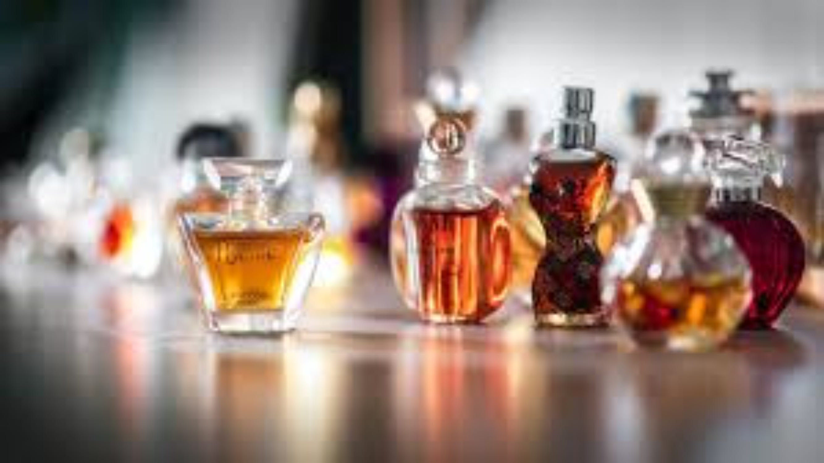
1. Smell of perfume spreading across the room:

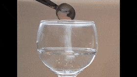
2. Sugar dissolving and spreading uniformly in water:

There are some properties which the diffusion process carries:

1. Structure slowly disappears

2. Things become more uniform and noisy over time

But why are we discussing about this now?

The main question is that can we do something similar with our data as well?

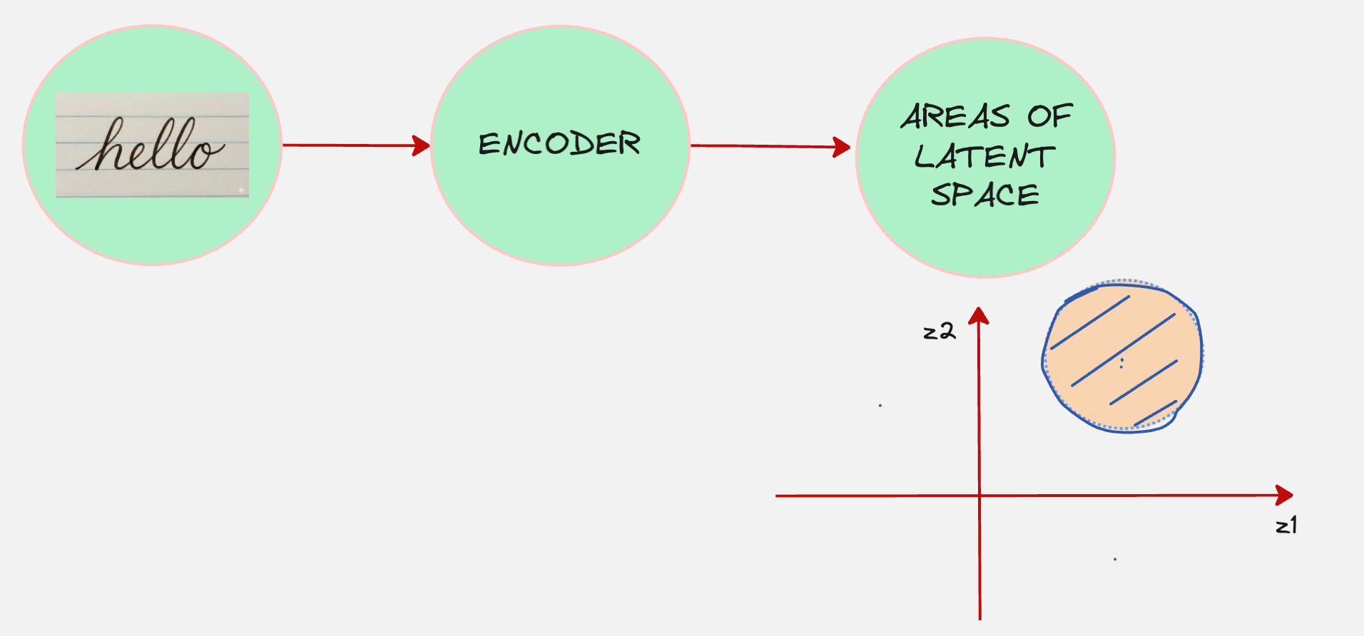
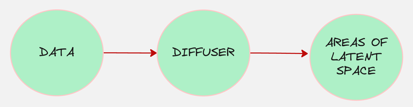
Remember that in the variational autoencoder, our encoder took the data as the input and then converted that into a representation in the latent space.

Refer to this article on Variational AutoEncoders: https://www.vizuaranewsletter.com/p/variational-autoencoders-explained

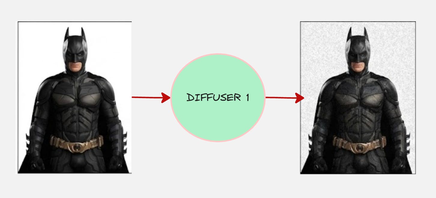
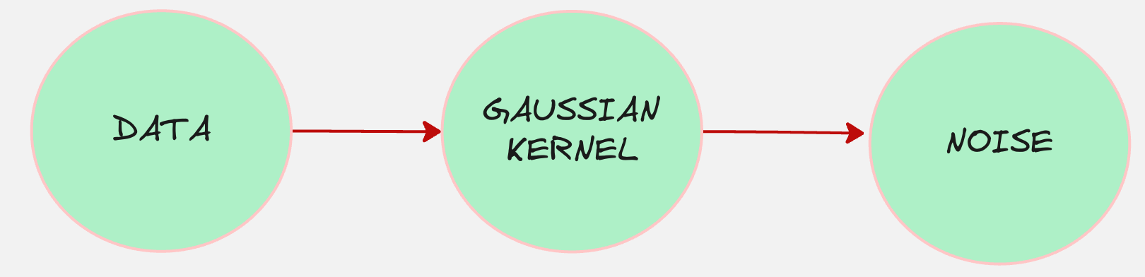
What if we think of our encoder as a machine which diffuses the data?

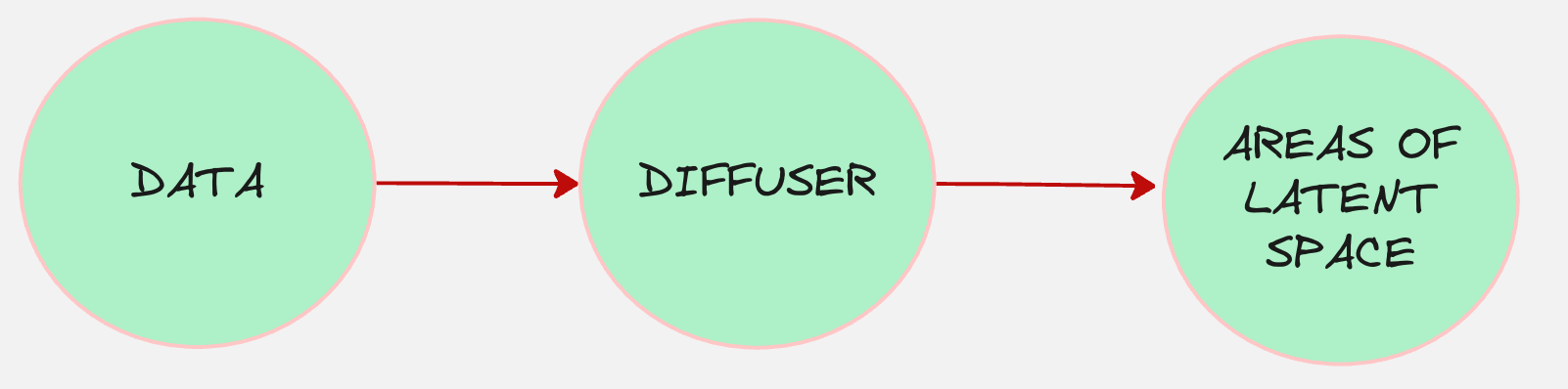
And the diffuser works such that it converts the data into pure noise.

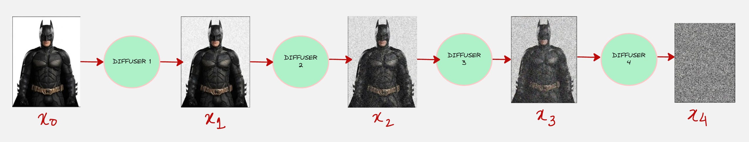
Let us take an example

Consider this image:

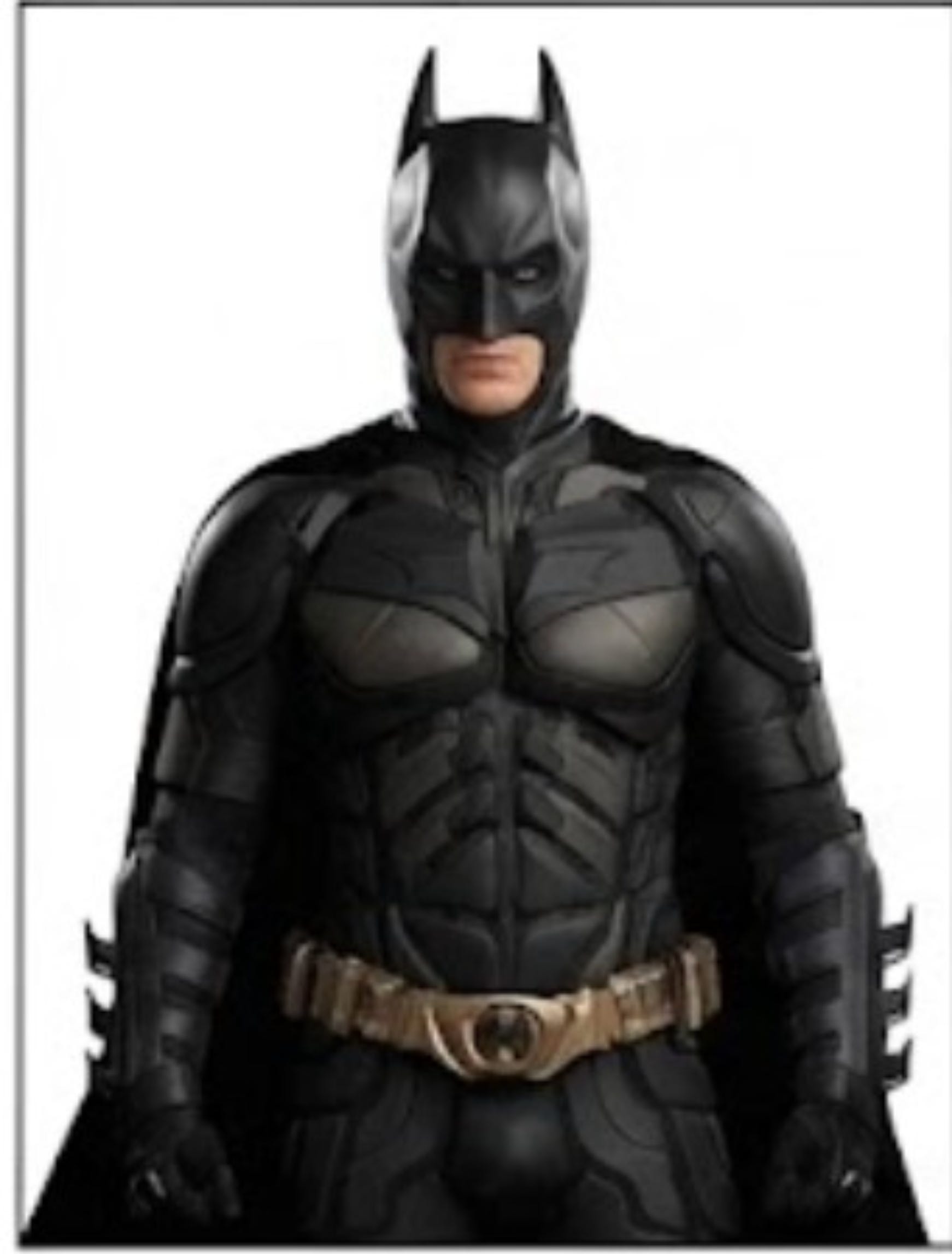
Yes, we are taking Batman as our example :)

The encoder will do something as follows:

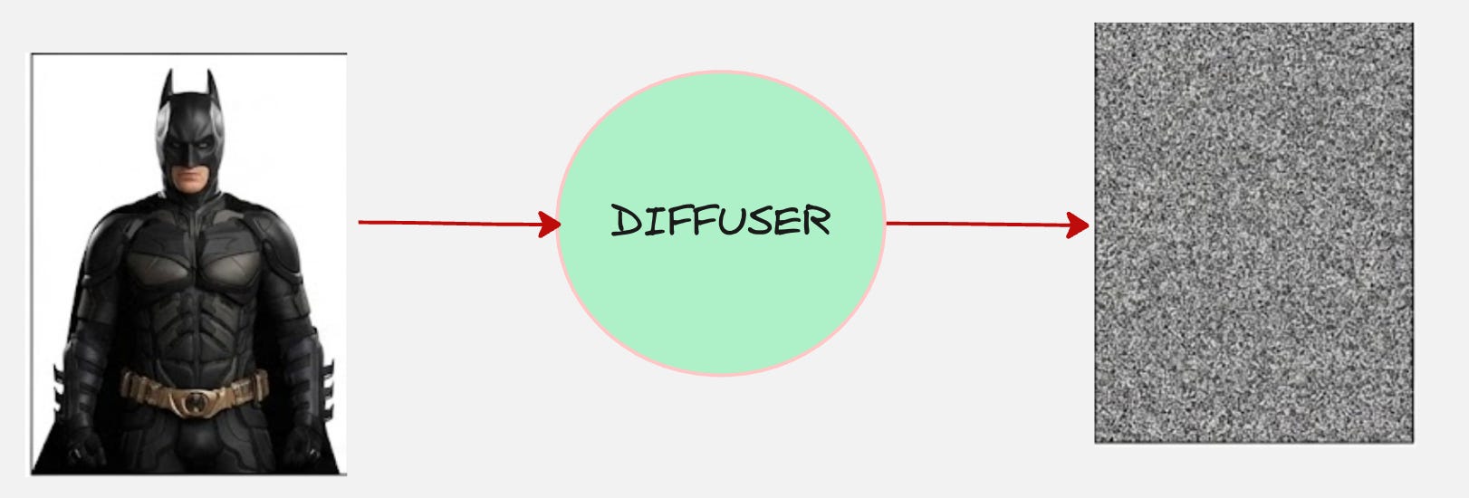
We will make one additional change, instead of directly transforming the image into noise, we will make the transformation gradual.

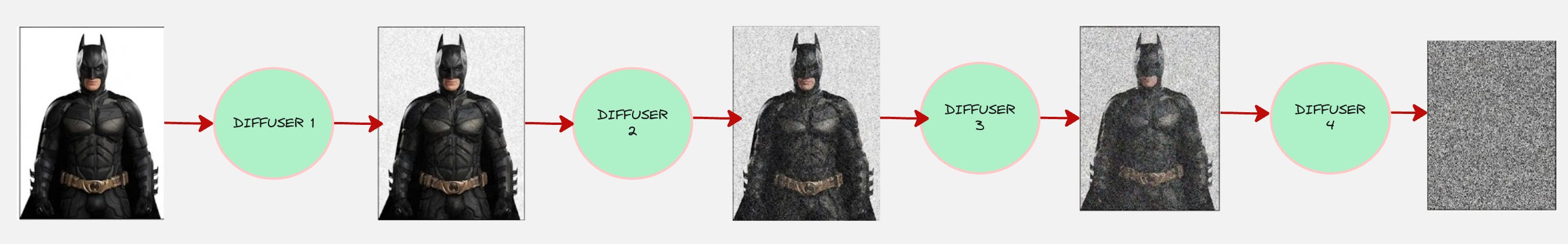
So, there are multiple encoders which we need to train?

Remember, this was one of the drawbacks of VAEs, where both the encoder and decoder had to be trained simultaneously

What if we fix these encoders/diffusers?

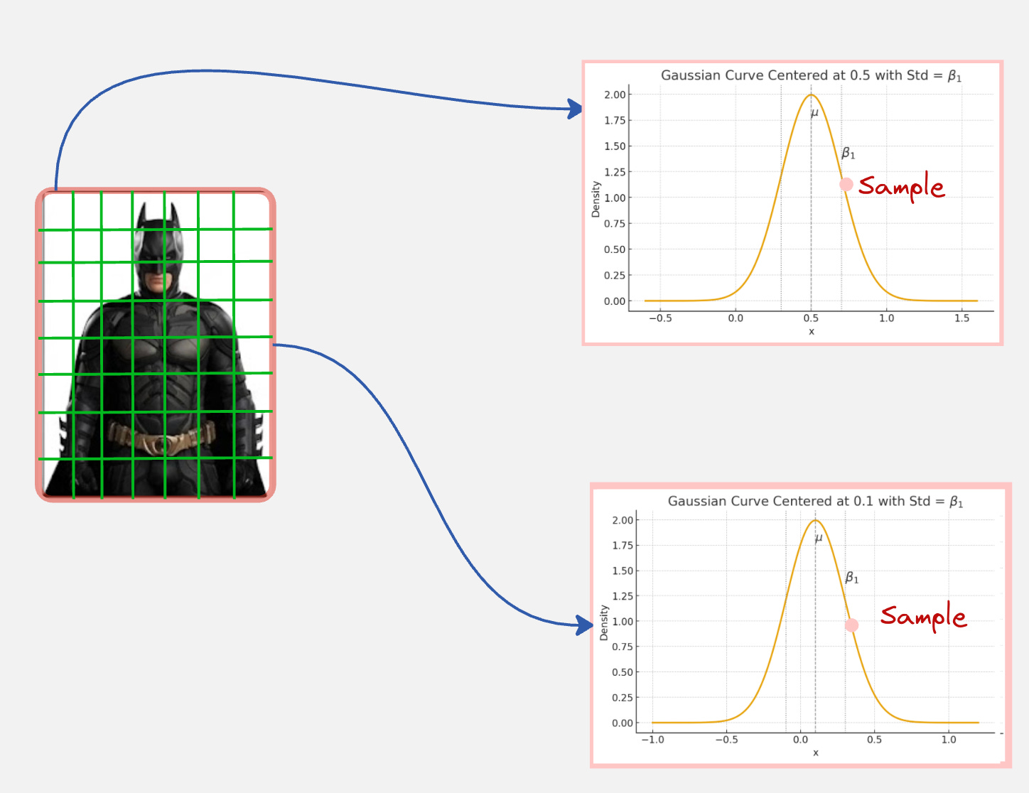
Let us say we modify our Batman image by adding a fixed Gaussian Kernel.

We can represent our image first a grid of pixels.

These pixels have some fixed values.

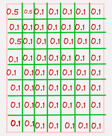
Now, for each pixel, we will sample from a Gaussian with the mean fixed to be the pixel value and a small variance (beta).

This will look something like below:

What will happen if we do this for all the pixels?

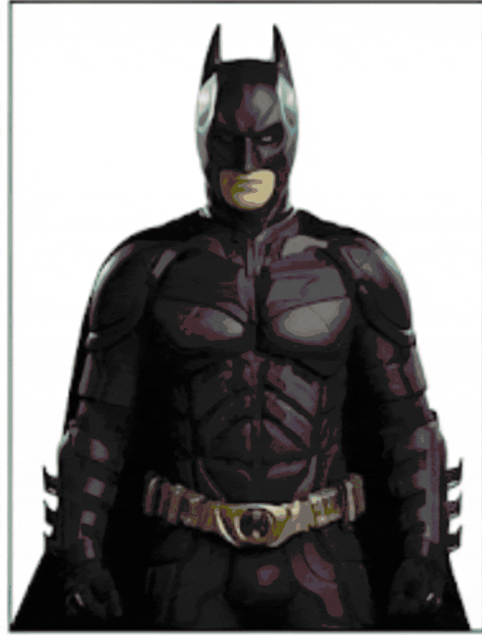
If we do this process to all the pixels, we will get something like this:

This is a “noisy version” of the original Batman image.

What we did is also called as adding Gaussian Noise to the image

The mathematical representation for this can be written as:

\(x_{1} = x_{0} + \beta \epsilon\)

Here, x0, x1 and beta represent the original image, transformed image and the standard deviation respectively. Epsilon denotes a random variable which can take any value between 0 and 1.

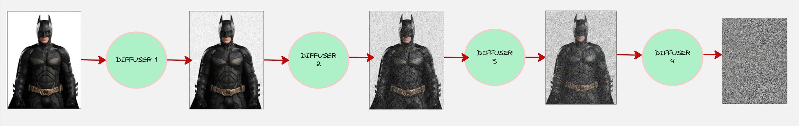
Now, what will happen if you do this a large number of times?

This is what you get:

There is one problem with the above method though. If you observe the animation closely, you will realize that we are adding a lot of noise, but the original image is preserved as it is.

This is different from the definition of “Diffusion” which we started out with:

1. Structure slowly disappears

2. Things become more uniform and noisy over time

This happens because we are preserving the mean value of the pixels. The structure will slowly break down when the mean also changes and move towards 0.

Remember that we want to achieve this:

Our current “diffuser” does not achieve this.

Let us do this: For each “diffuser”, we will also scale the mean down by some factor along with injecting noise.

Something like this:

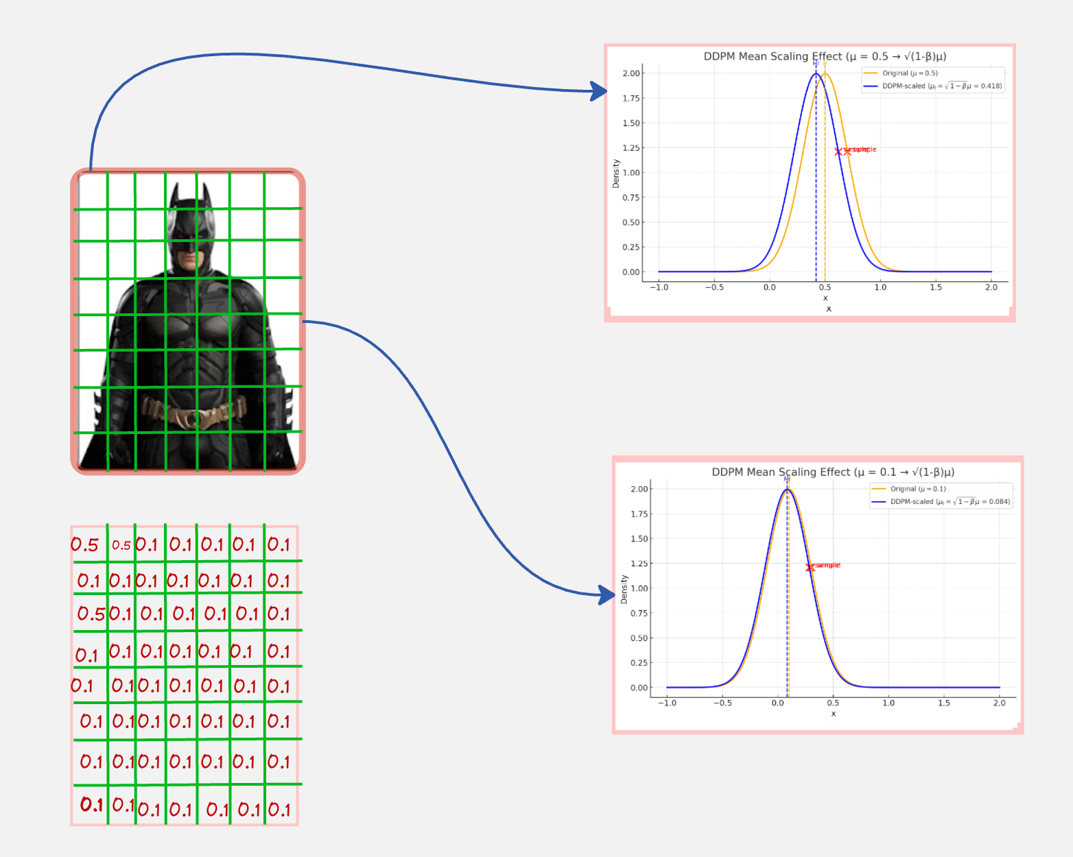
Notice how for the 2 pixels, we are sampling from a distribution with a mean which is scaled down (such that it moves towards zero).

The mathematical representation for this can be written as:

Okay, this is looking good. But, we have multiple diffusers (4 in the diagram above). Let us how we transform the original image to the final image mathematically:

Okay this makes sense.

But there is one small thing left:

The noise is not kept constant for all transitions. The noise schedule is kept such that it increases as we transform the clean image to noise.

Also, the mean is chosen such that the square of the mean and the standard deviation is equal to 1. This is done so that the total variance at every step remains constant and also to ensure numerical stability across time steps.

So, the transitions can now be written as follows:

\(x_{1} = \sqrt{1-\beta_{1}^{2}} x_{0} + \beta_{1} \epsilon\)

\(x_{2} = \sqrt{1-\beta_{2}^{2}} x_{1} + \beta_{2} \epsilon\)

\(x_{3} = \sqrt{1-\beta_{3}^{2}} x_{2} + \beta_{3} \epsilon\)

\(x_{4} = \sqrt{1-\beta_{4}^{2}} x_{3} + \beta_{4} \epsilon\)

Now, what will happen if you do the same thing large number of times?

This is what you get:

This is exactly what we want!

Reiterating our approach, we can now express this diffusion process as follows:

“For every pixel in the image, sample from a Gaussian distribution. The mean of the Gaussian distribution should be scaled by a factor of alpha, and the standard deviation should be beta.”

We do this for every transition. So, our forward diffusion process looks as follows:

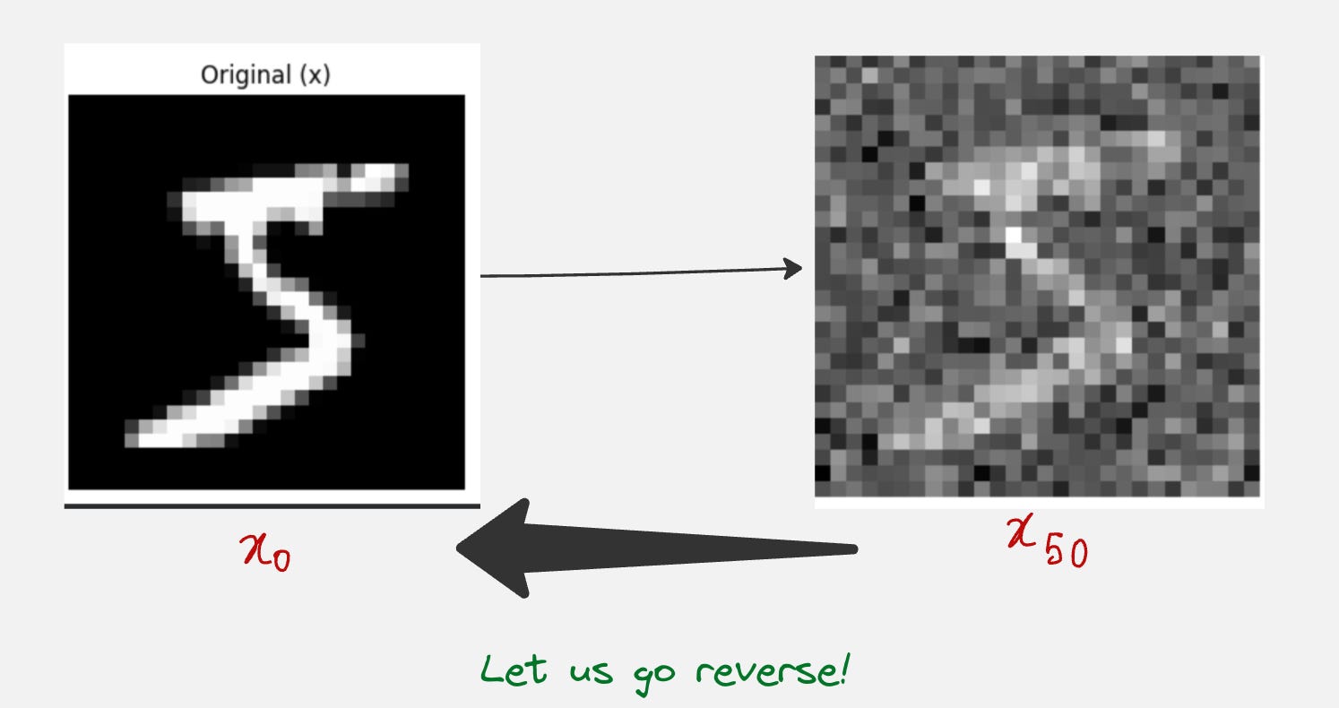
Let us take a look at a practical example of applying the forward diffusion process to simple English Letters.

We will transform the letter “T” to noise using the forward diffusion process.

Here is the link to the Google Colab notebook:

Application of the forward diffusion process to a practical example

So our choice of the Gaussian transition kernel actually works!

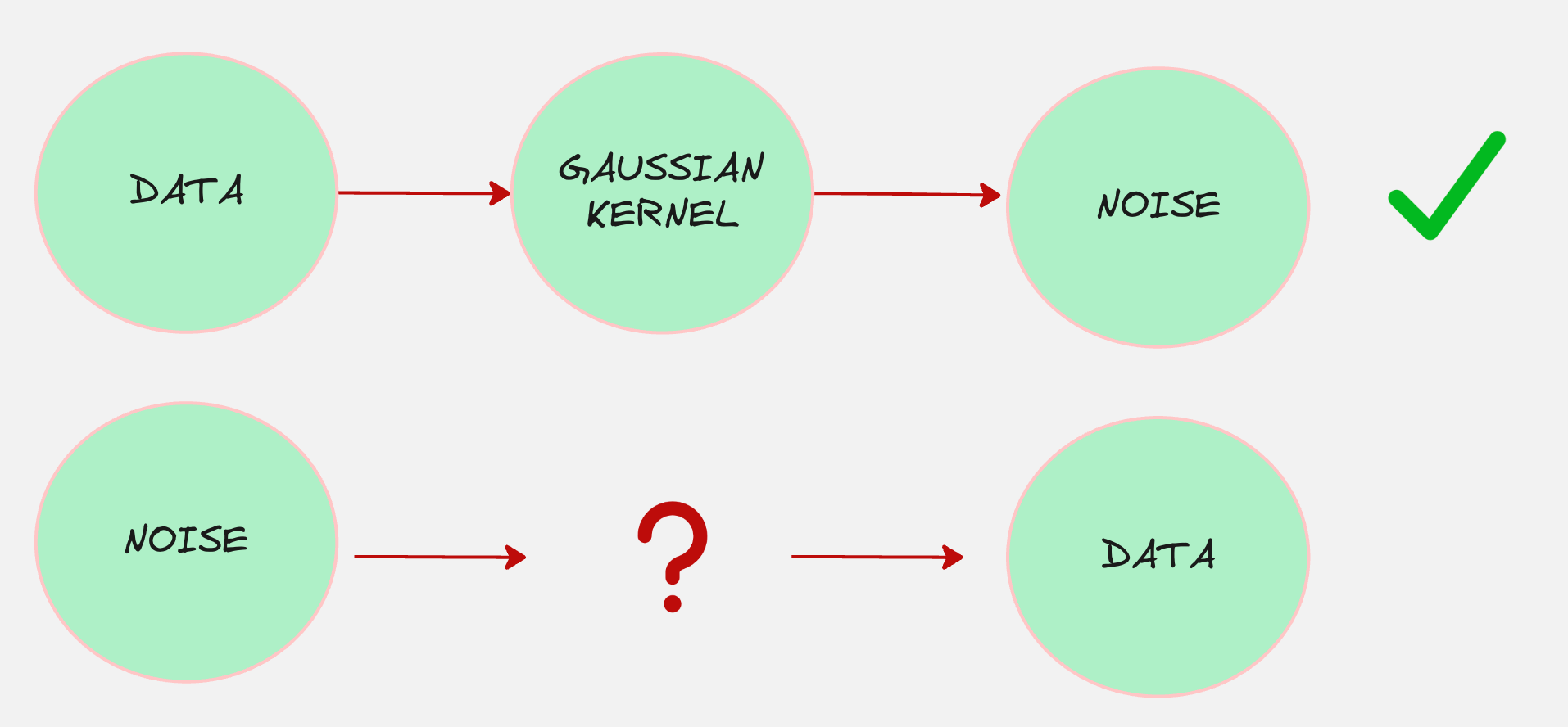
Remember we started out with the following:

What if we think of our encoder as a machine which diffuses the data?

Now, we have completely defined the above process which looks as follows:

But the main question remains:

(1) What about the decoder? How does it look like?

(2) And how can we learn the original data distribution?

The Learnable Decoder

Our objective is to starting from pure, unstructured noise and to progressively denoise this randomness, step by step, until a coherent and meaningful data sample emerges.

For example, if the true data distribution is that of cats, then this process would look something as follows:

The decoder distribution is denoted as:

\(p_{\theta}(x)\)

Whatever we do in this reverse process, the final goal is to maximize the probability of sampling the images from the true data distribution.

So, our objective is the following:

\(max[p_{\theta}(x_{0})]\)

This also means that we want to maximize the following:

\(max[\text{log}(p_{\theta}(x_{0}))]\)

Just as we did for VAEs, we can calculate the lower bound for this quantity as follows:

\(\text{log}(p_{\theta}(x_{0})) > E\)

It can proved that, here E is given by the following expression:

\(E = \text{log}p_{\theta}(x_{0}|x_{1}) - D_{KL} (p(x_{T})|q(x_{T}|x_{0})) - D_{KL}[p_{\theta}(x_{t-1}|x_{t}) | q(x_{t-1}|x_{t},x_{0})]\)

Here, ‘T’ denotes the last time-step in the forward diffusion process, when the data becomes noise.

“q” denotes the true posterior, which means the actual conditional distribution implied by the real generative process, not an approximation made by your model.

The three terms can be denoted as “Reconstruction”, “Regularization” and “Matching the Reverse Distribution”

The first 2 terms are very similar to what we saw in the variational autoencoders. For the training of diffusion models, we ignore the first two terms and only focus on the third term.

The third term is an extra term here, which basically means that the predicted reverse transition distribution should match as close as possible to the true transition distribution (also known as the true posterior).

Let’s take an example:

In the above image, you can see an example of a handwritten note which is smudged because of the rain.

Now, the main question is the follows?

Can we predict the image at the previous time step, x(t-1)?

The problem here is that, we do not know the reverse process? We cannot just go back in time :(

Now consider another case: Suppose you knew the image which you started out with, the original image.

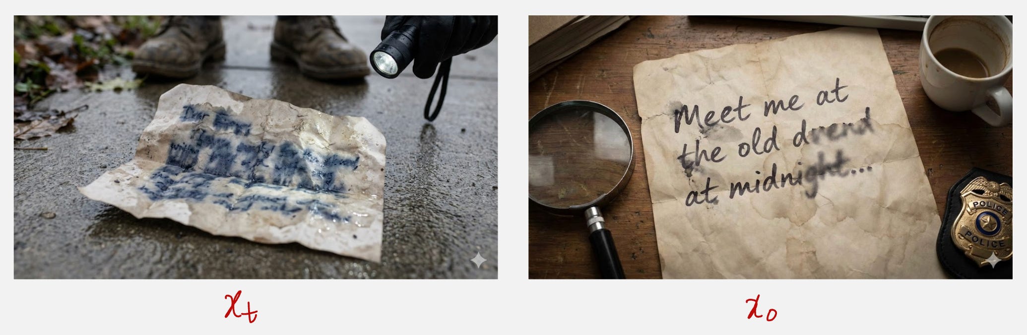
Now, suddenly it becomes much easier to find the image at the previous time step, which is x(t-1). This is because we have access to the original image.

Okay, still, how can do this, even if we have the original image?

The question we are asking is:

If we knew the image of the Batman at one time step and we knew the original image, can we find the image of the Batman at a previous time step?

We want to find the true posterior, given by (if we consider the third time step):

\(q(x_{2}|x_{3},x_{0})\)

The way I think about it is that:

In three time steps, I have to reduce the noise by this much. So in one time step, I will reduce the noise by one-third of that amount.

It turns out that this reverse process can be approximated by a Gaussian distribution with a mean and a variance.

Intuitively, we expect the mean to depend on the original image as well as the image at the current time step.

Hence, we can write the mean of the true posterior as follows:

\(\mu (x_{i},x_{0}) = A_{1}x_{0} + A_{2} x_{i}\)

Here, xi denotes the current image and x0 denotes the original image.

Here, A1 and A2 are functions of the standard deviations in the forward transition process. I will include a book in the resources section where you can find the derivation for these values.

\(A_{1} = f(\beta_{1},\beta_{2},\beta_{3}...)\)

\(A_{2} = g(\beta_{1},\beta_{2},\beta_{3}...)\)

The standard deviation of the true posterior can also be written as a function of all the standard deviations, which can be denoted as follows:

\(\sigma(i) = A_{3}\)

Let us look at a practical example where we apply the mathematical form for the true posterior to transform a noisy image into an original image, given the original image as the input.

Here, we will take the example of handwritten digits.

Here is the link to the Google Colab notebook:

Application of the true posterior gaussian distribution formula to a practical example

A question for all of you to think about: How does A1 and A2 change as the reverse transition process proceeds? Do they increase or decrease in magnitude as we go closer to the true image?

A thought might come to your mind which says that we know the entire reverse process now: So are we done?

Well, not quite. The reason is that we have calculated the reverse transition kernel conditioned on the original image.

In our application, we have to generate the image from the noise, so the original given image will not be known to us.

Look at the third term in our objective function, which we want to maximize:

\(- D_{KL}[p_{\theta}(x_{t-1}|x_{t}) | q(x_{t-1}|x_{t},x_{0})]\)

This means that we need to minimize the KL divergence between our model prediction and the true posterior.

Our true posterior is a Gaussian, and we will assume that our model prediction is also a Gaussian distribution. The mean of our model distribution is not known to us. However, we will assume that our model has the same variance as that of the true posterior.

This means that our task is to minimize the KL divergences between two Gaussians with the same variance and different means.

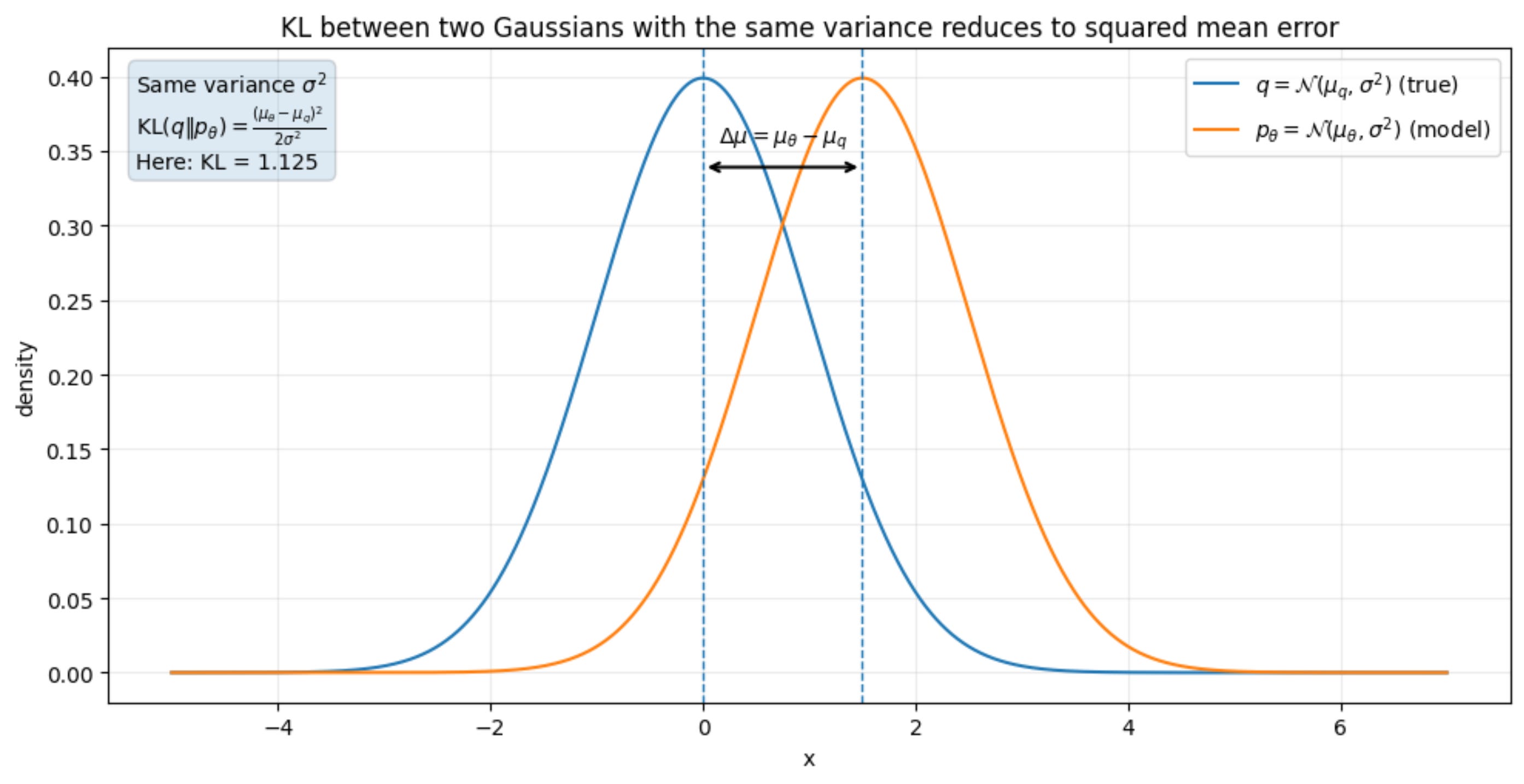
It turns out that this is equivalent to minimizing the mean square error between both the means:

\( D_{KL}[p_{\theta}(x_{t-1}|x_{t}) | q(x_{t-1}|x_{t},x_{0})] = \frac {1}{2\sigma^{2}}||\mu_{\phi}(x_{i}) - \mu(x_{i},x_{0})||^{2}\)

Now, let us see how we can simplify this loss:

We already know the mean of the true posterior:

\(\mu (x_{i},x_{0}) = A_{1}x_{0} + A_{2} x_{i}\)

Let us approximate the mean of our model to be as follows:

\(\mu_{\phi} (x_{i}) = A_{1}\hat{x_{0}} + A_{2} x_{i}\)

Now our loss function can be written as follows:

\( D_{KL}[p_{\theta}(x_{t-1}|x_{t}) | q(x_{t-1}|x_{t},x_{0})] = \frac {A_{1}^{2}}{2\sigma^{2}}||\hat{x_{0}} - x_{0}||^{2}\)

This means that:

To make our one-step reverse distribution match the true one, it’s enough to make our predicted clean sample​ close to the real one.

So training becomes a simple supervised regression problem: predict the clean thing from the noisy thing.

Now, we can do one more simplification to make it even more intuitive.

The real clean sample can be predicted from the real current image by removing noise.

The predicted clean sample can be predicted from the predicted current image by removing the predicted noise.

This means that we can express the real clean sample and the predicted clean sample in terms of the real noise and the predicted noise

After doing this, the last term simplifies to the following:

\(D_{KL}[p_{\theta}(x_{t-1}|x_{t}) | q(x_{t-1}|x_{t},x_{0})] = C||\hat{\epsilon} - \epsilon||^{2}\)

Here, C is a constant.

This means that:

To make our one-step reverse distribution match the true one, it’s enough to make our predicted noise​ close to the real noise.

That’s it!

Here is the link to the original paper which introduced DDPM (Denoising Diffusion Probabilistic Models): https://arxiv.org/abs/2006.11239

For more detailed proofs, please refer to the book: The Principles of Diffusion Models From Origins to Advances (https://arxiv.org/abs/2510.21890) [Pages 43-55]

If you like this content, please check out our bootcamps on the following topics:

Modern Robot Learning: https://robotlearningbootcamp.vizuara.ai/

GenAI: https://flyvidesh.online/gen-ai-professional-bootcamp

RL: https://rlresearcherbootcamp.vizuara.ai/

SciML: https://flyvidesh.online/ml-bootcamp

ML-DL: https://flyvidesh.online/ml-dl-bootcamp

CV: https://cvresearchbootcamp.vizuara.ai/