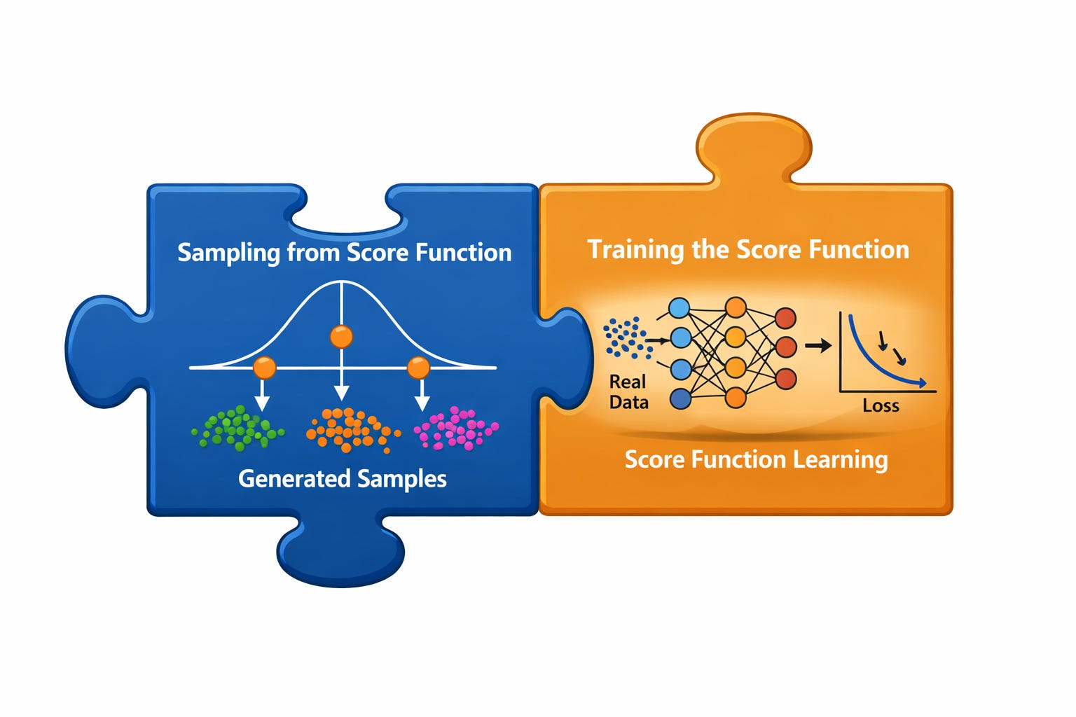
Energy Based Models - Score Matching

Modeling probability distributions using energy functions.

EBMs define a probability density via an energy function which assigns lower energy to more likely configurations.

The Energy Function is represented as:

\(E_{\phi}(x)\)

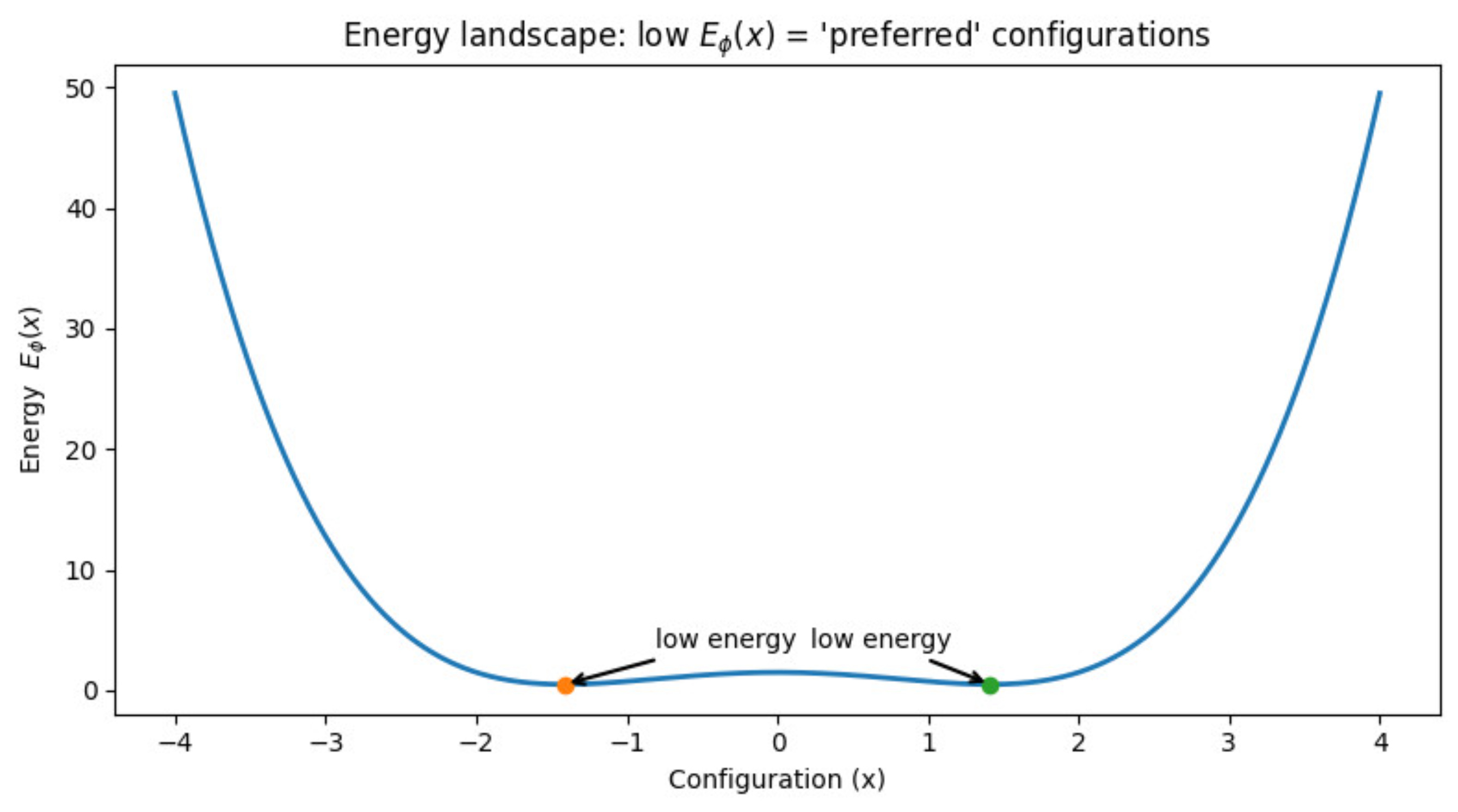
Let us look at a simple example:

Now, let us understand how do we think of converting this energy function into a probability distribution.

Some things which we understand intuitively are:

The points with low energy should have a higher probability.

The points with high energy should have a lower probability.

This is inspired from physics, where we see that the systems always reach a point of the lowest energy value. Think of an apple which is dropped from a height. The reason it settles on the ground is because the potential energy there is the minimum.

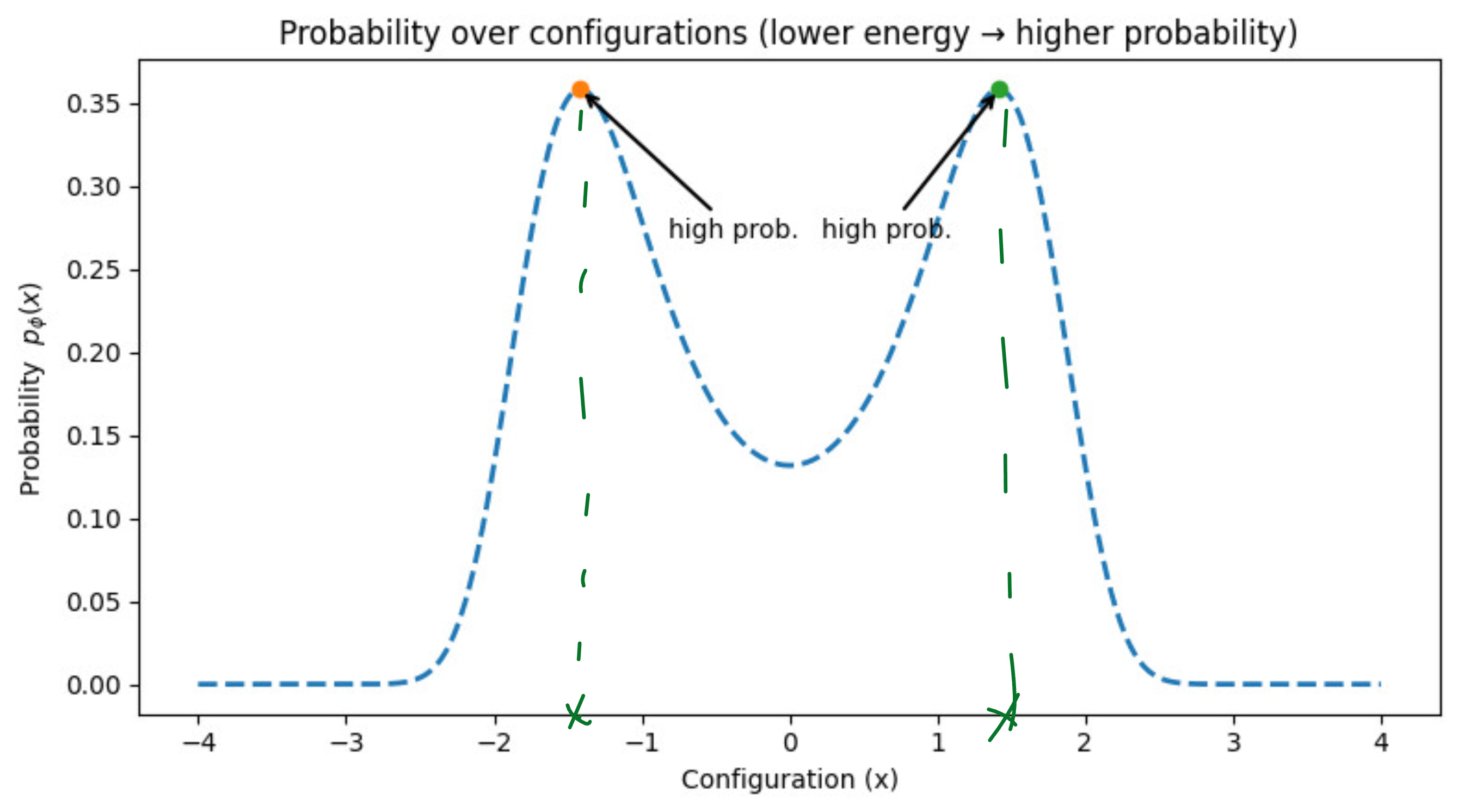
So, the probability curve should look something like this:

Let us superimpose both the curves now:

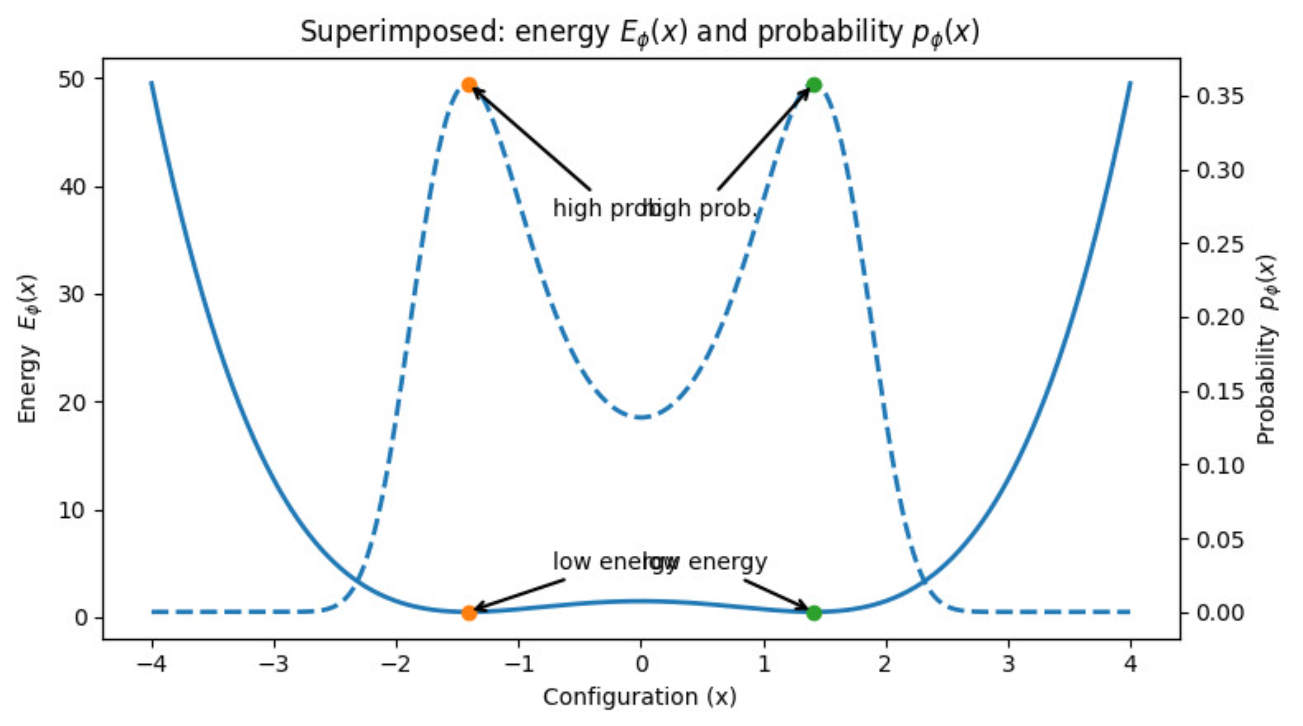
This is what we want.

Can we think of a mathematical function which takes us from this energy curve to the probability curve?

The function should satisfy the following properties:

• Higher energy should have lower probabilities

• Lower energy should have higher probabilities

• Should have only positive values

• Should lie between 0 and 1

People use an exponential function to relate the energy to the probability since it satisfies all these properties.

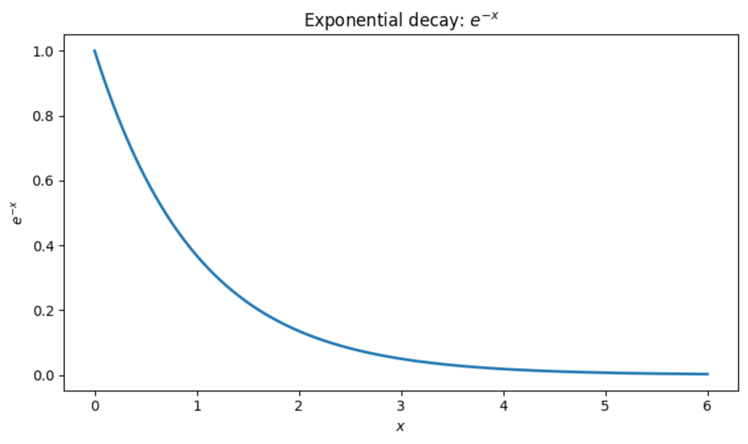
From the above graph, we can relate the energy to the probability using the following equation:

\(p_{\phi}(x) = e^{-E_{\phi}(x)}\)

Okay, this looks great, until it is not..

Let us look at an example:

Let us take an example. Suppose that we have a set of discrete states which are -3, -2, -1, 0, 1, 2, and 3.

Now, let us say we use the above formula and calculate the probability densities for all these states.

It will look something like this:

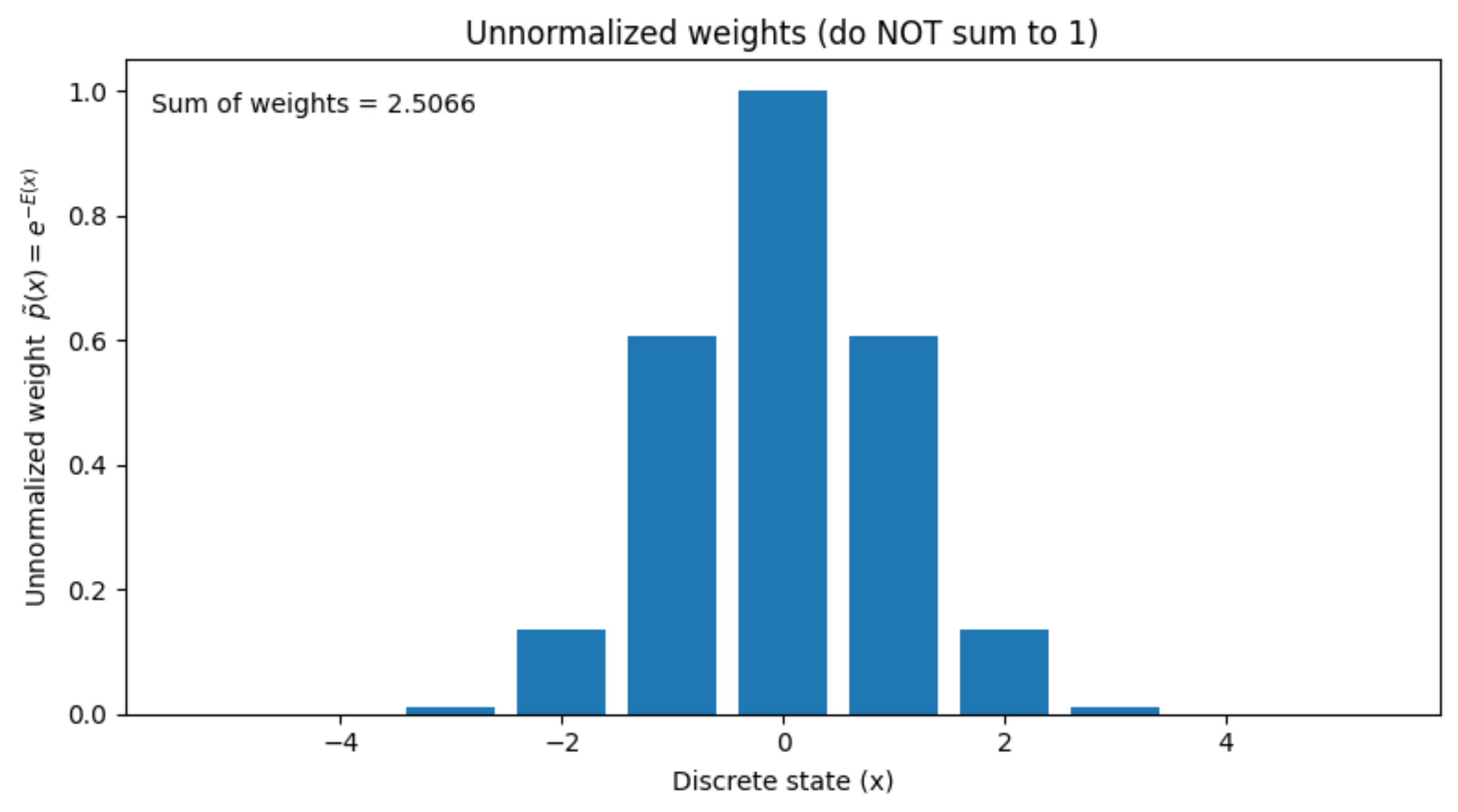
Here, we are assuming that the energy function for all these states is known to us, and we are simply converting them into probability using the exponential formula, which we looked at before.

The sum of all these probabilities is 2.5066.

This is not what we want. We want the summation of all the probabilities to be 1, so that it is an actual probability density function.

However, there is a simple solution to this. We can simply normalize the probabilities by dividing it by 2.5066.

It will look something like this:

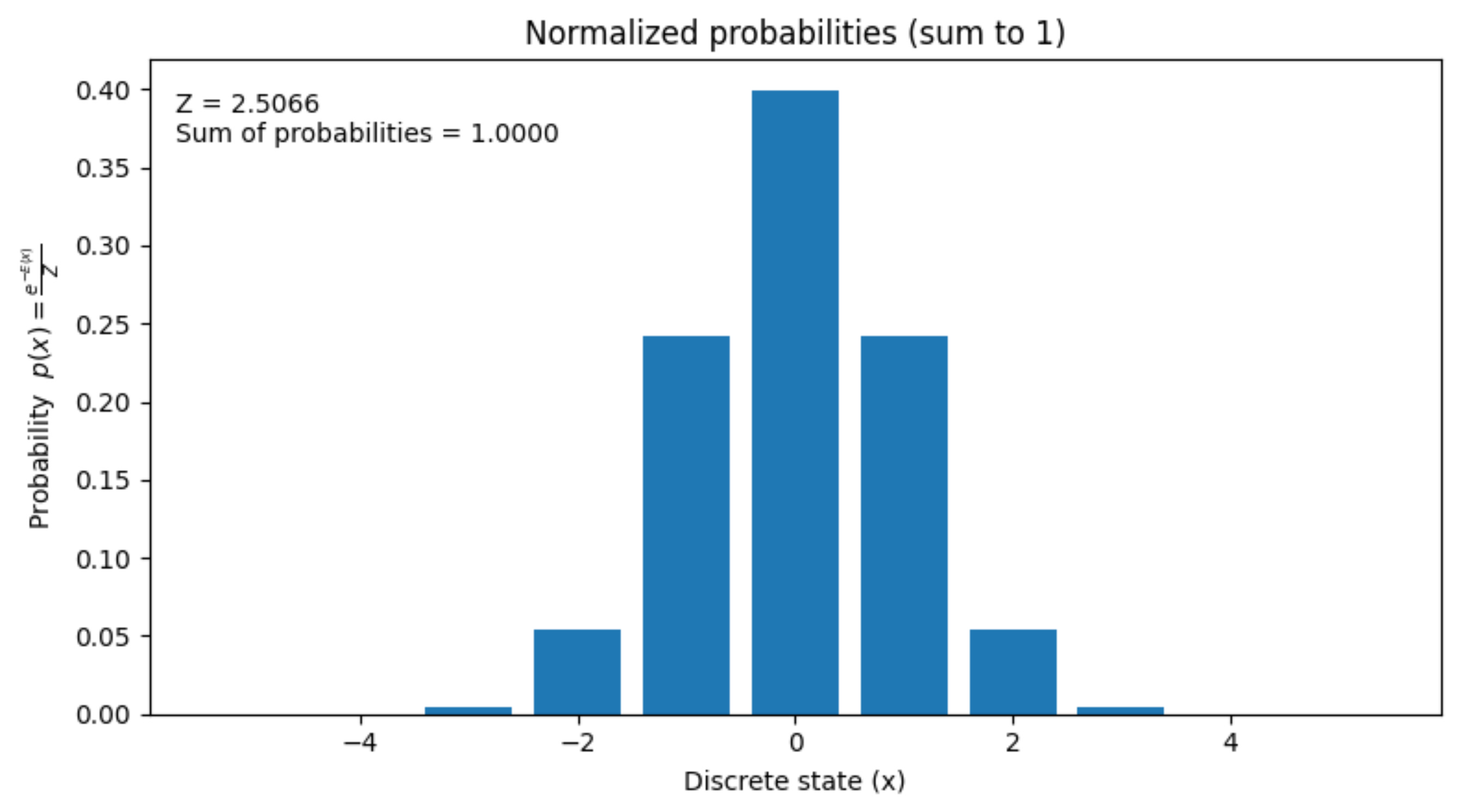
Now, these probabilities do sum up to 1!

The number 2.5066 is called as the partition function.

Hence the final relation between energy and the probability density function will look as follows:

\(p_{\phi}(x) = \frac{e^{-E_{\phi}(x)}}{\int e^{-E_{\phi}(x)} dx }\)

The partition function, which is the denominator in the above equation is also denoted by the symbol “Z”.

This is great, but how do we train Energy-based models?

Training Energy-Based Models

Conceptually, we want to do something like this:

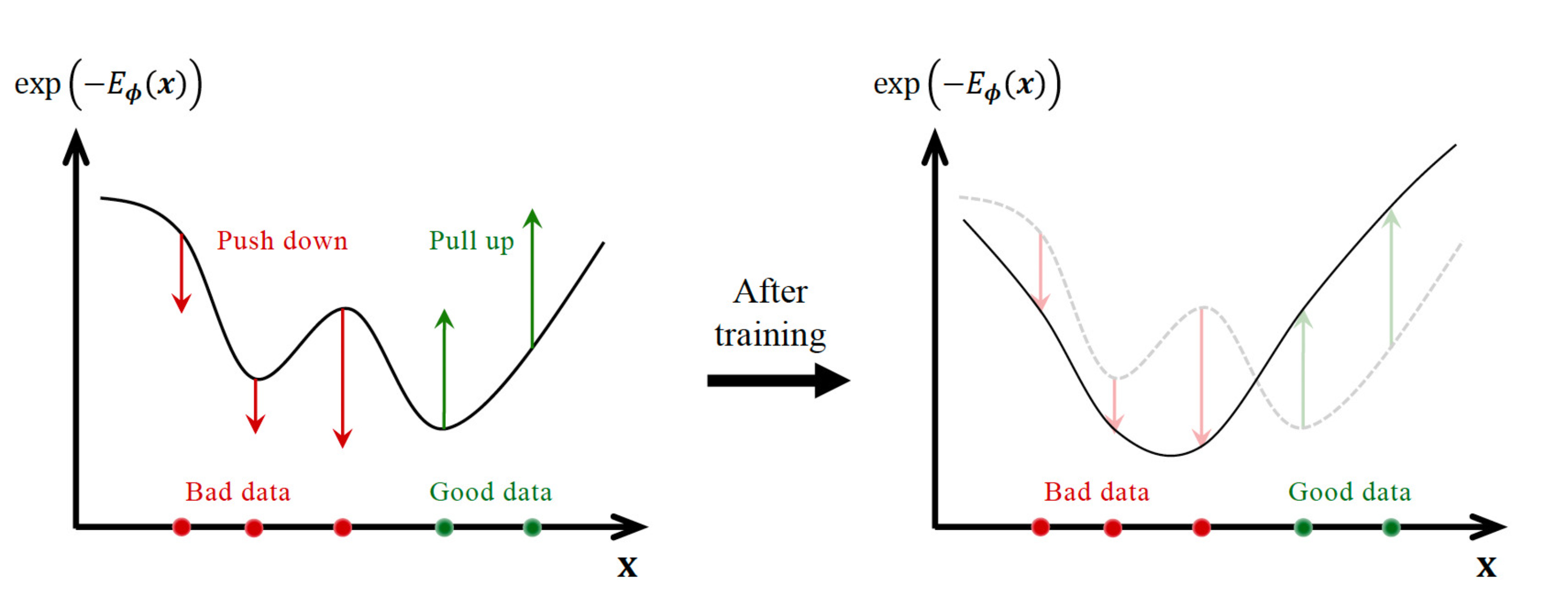
We start with the random energy configuration and slowly modify the energy landscape, so that the bad data have a lower probability and the good data have a higher probability.

We will again use the maximum likelihood which we have seen before multiple times.

We want to maximize the following:

\( \text{log}p_{\phi}(x)\)

Using the above formula, which relates the energy to the probability, we can rewrite the above equation as follows:

\( \text{log}p_{\phi}(x) = -E_{\phi}(x) - log(Z)\)

Here, Z denotes the partition function.

The main challenge with the above equation is that the partition function is intractable, i.e., it is impossible to calculate it. The reason is that we do not know the energy function for all the states in the distribution, and calculating an integral over all of them is impossible.

Remember we had faced this same issue while training variational autoencoders and diffusion models as well.

We had solved those issues by formulating an ELBO term and then maximizing that ELBO term. This worked for us because the ELBO term is always less than the maximum likelihood.

For energy-based methods, we don’t use the ELBO approach, but instead we introduce the notion of the score function and present score matching as a tractable training objective which bypasses the partition function.

What is the “Score”?

The score function is the gradient of the log density, given by the following equation:

\(s(x) = \nabla_{x}\text{log}p(x)\)

Here, p(x) denotes the probability distribution of the data.

Intuitively, the score forms a vector field that points toward regions of higher probability, providing a local guide to where the data is most likely to occur

In the above figure, the arrows represent the score field which are pointed towards the direction where the density of the data is the maximum.

The score function acts as a compass, guiding you towards areas where the probability of the data being from the distribution is the maximum.

Let us look at a simple practical example to build our intuition about the score function.

Let us assume that the probability density curve is Gaussian.

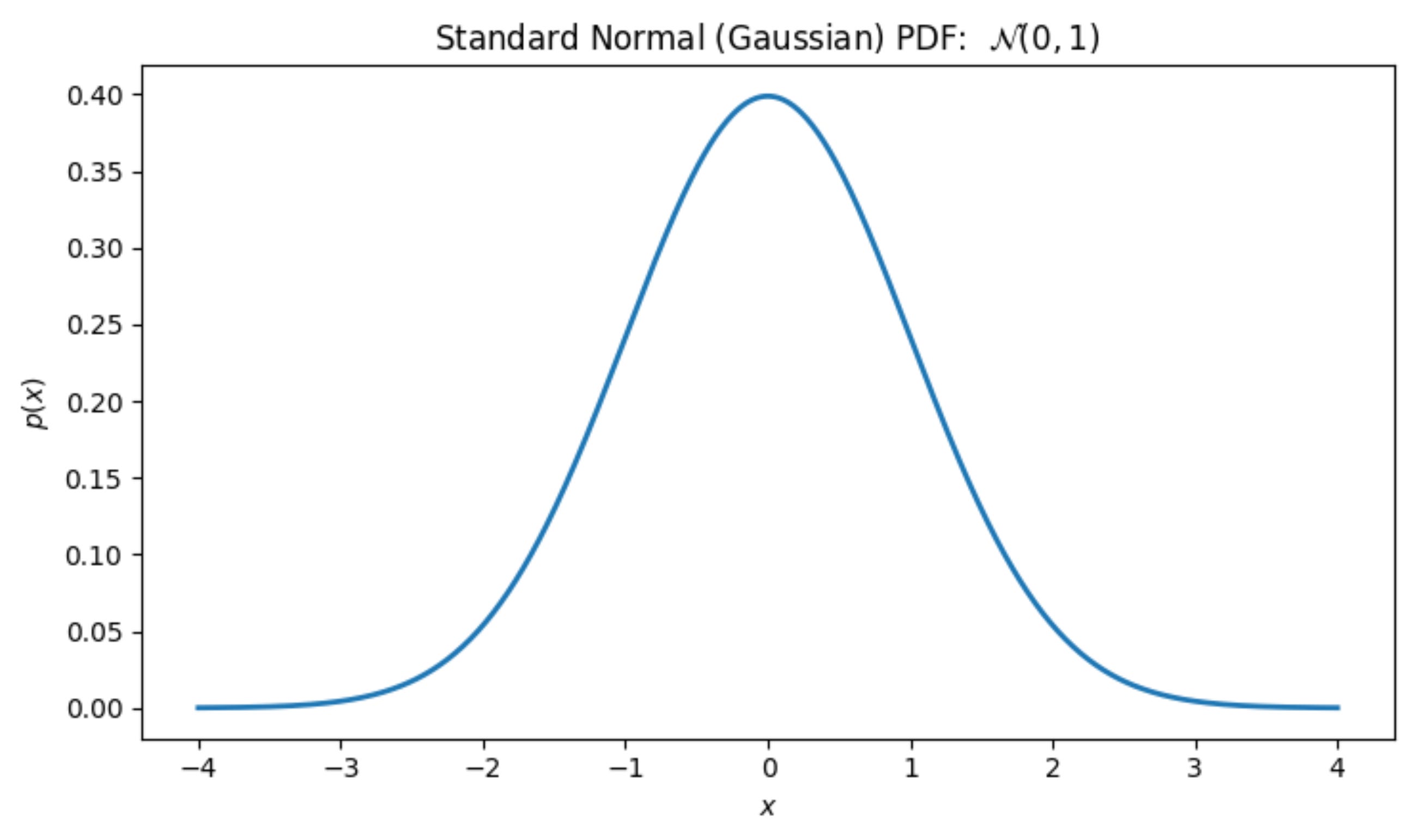
First, let us write down the mathematical functional form for the Gaussian:

\(p(x) = \frac{1}{\sqrt{2\pi}}e^{-x^{2}/2}\)

We can verify whether this makes sense. If we substitute x = 0, we get a positive value for the probability, and for very high values (positive or negative), the probability becomes 0, which matches the graph above.

Now, let us calculate the score function.

First, let us calculate the logarithm of the probability:

\(\text{log}(p(x)) = \text{log}(\frac{1}{\sqrt{2\pi}}) - \frac{x^{2}}{2}\)

Now, we will take the gradient. The gradient of the constant will vanish.

\(s(x) = \nabla_{x}\text{log}(p(x)) = -x \)

Let us visualize this score function superimposed on the probability density curve:

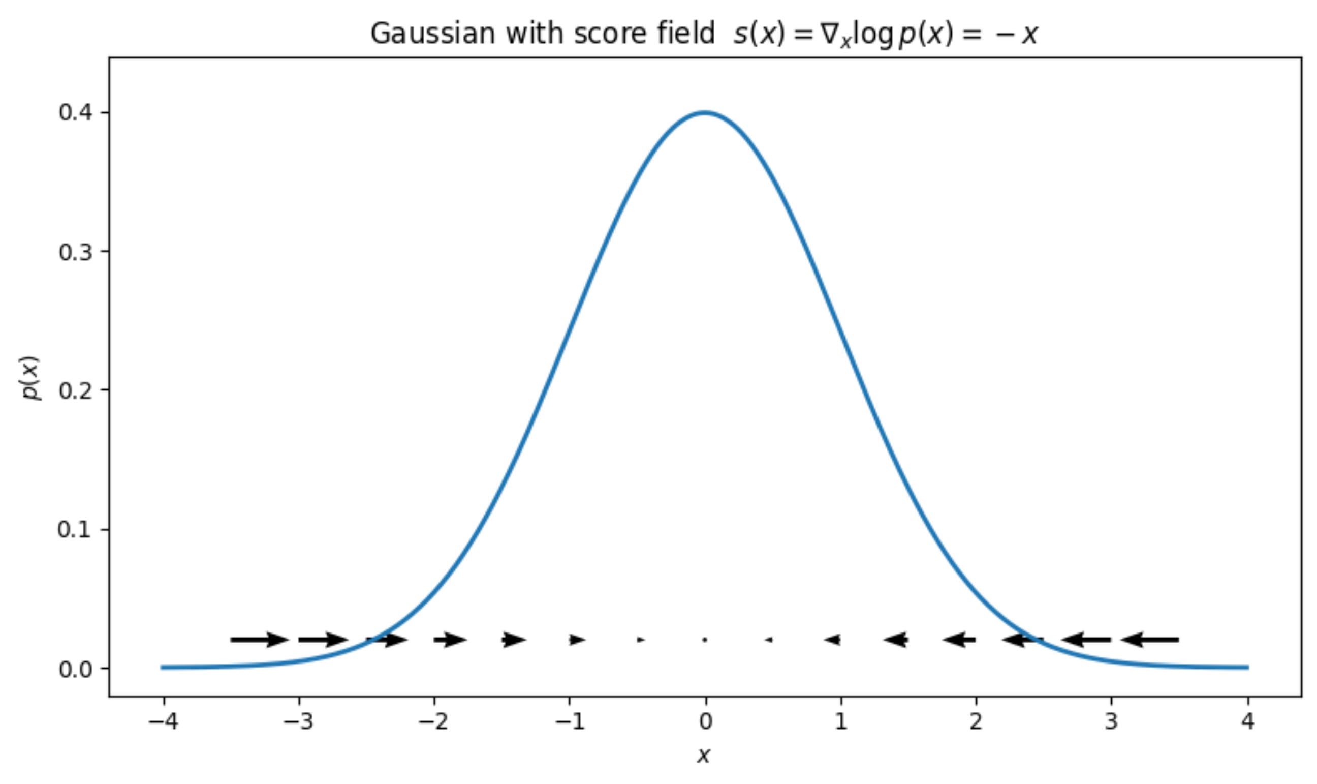
In this example, we can clearly see that all the score vectors are pointed towards the center because the origin has the maximum probability density.

The further you are from the center, the magnitude of the arrows increases because it is farther away, and it will require more force to pull it back to the center.

But why model scores instead of densities?

Modeling the score offers both theoretical and practical benefits:

Freedom from Partition Function:

We had seen before that calculating the partition function was intractable.

Because of this, we could not find an expression for maximizing the probability density likelihood.

Now, let us see how this formulation changes for the score function.

Let us write down the formula for the score function and substitute the probability with the energy function.

\(s(x) = \nabla_{x}\text{log}(p(x)) = \nabla_{x}\text{log}(\frac{e^{-E_{\phi}(x)}}{Z})\)

This can be simplified to the following. Remember the log of the exponential of a value is the value itself.

\(s(x) = -\nabla_{x}E_{\phi}(x) - \nabla_{x} \text{log}Z\)

Now the second term here involves calculating the gradient of the partition function, which does not depend on x. So that gradient will become zero, and this is exactly why we get the freedom from the partition function.

So, we can write the score function as follows:

\(s(x) = -\nabla_{x}E_{\phi}(x)\)

Now that we have understood the meaning of the score function, let us use this formulation of the score function for training energy-based models.

Before we go to the training of energy-based models using the score function, let us first understand how can we get samples from our distribution if we only know the score function.

Sampling using the Score Function

The question that we will address is, “How do you sample the data if you have the score function?”

Let us start with an example:

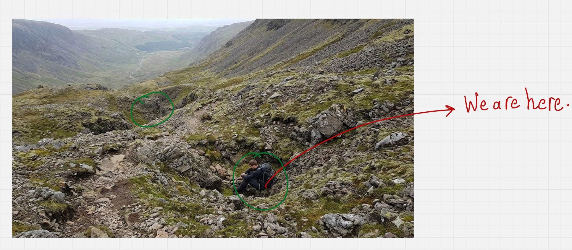
Imagine that you are dropped into a thick fog on a vast landscape. Your goal is to find the deepest valley because that is where the treasure is hidden.

Ideally, you want to trace the route which goes something like this:

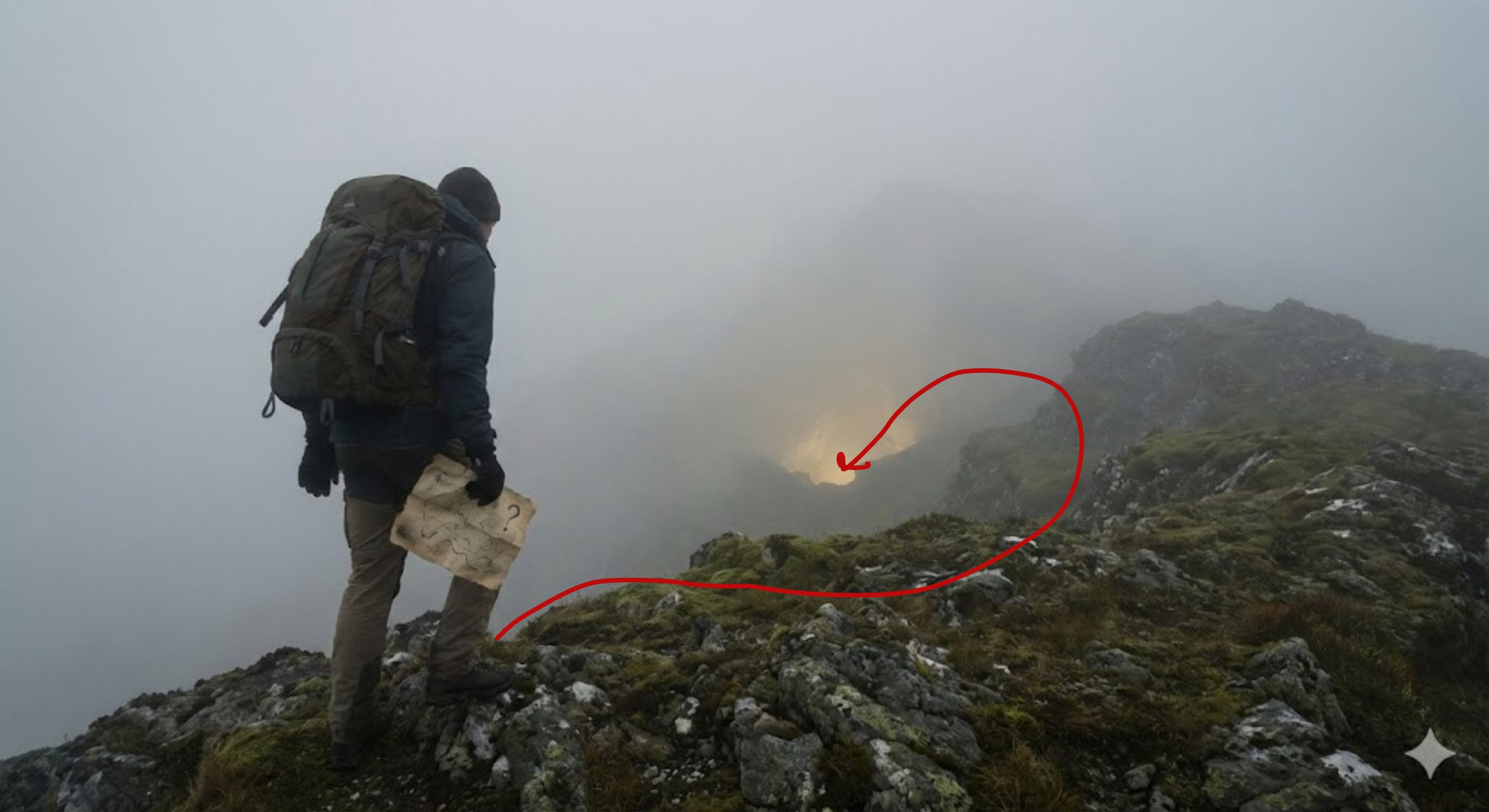
What is the strategy that you will use?

Since you know that the treasure is in the valley somewhere, you know that going down is good and going up is bad.

To reach the valley in the quickest possible time, you will go in the direction where the downward slope is the maximum.

Let us say the slope is given by the symbol “q”.

If x(t) is your current position and x(t+1) is your next position, then you can write the next position in terms of the current position using the following:

\(x_{t+1} = x_{t} + \eta q\)

Here, n is the step size.

In this analogy, our vast landscape is the energy function landscape. So, we are trying to find the point where the energy landscape achieves a minima.

So, the slope “q” can be expressed as the gradient of the energy function as follows:

\(q = - \nabla_{x} E_{\phi}(x_{t})\)

Note that we have used a negative sign because we want to find the minima, and not the maxima.

Now we can write the final update rule as follows:

\(x_{t+1}= x_{t} - \eta \nabla_{x} E_{\phi}(x_{t})\)

If we go according to the above rule, we are guaranteed to move towards regions where the energy function is minimum.

This would remind you of the “Gradient Descent Algorithm” in Machine Learning, where we have a very similar update rule.

We are not done yet :(

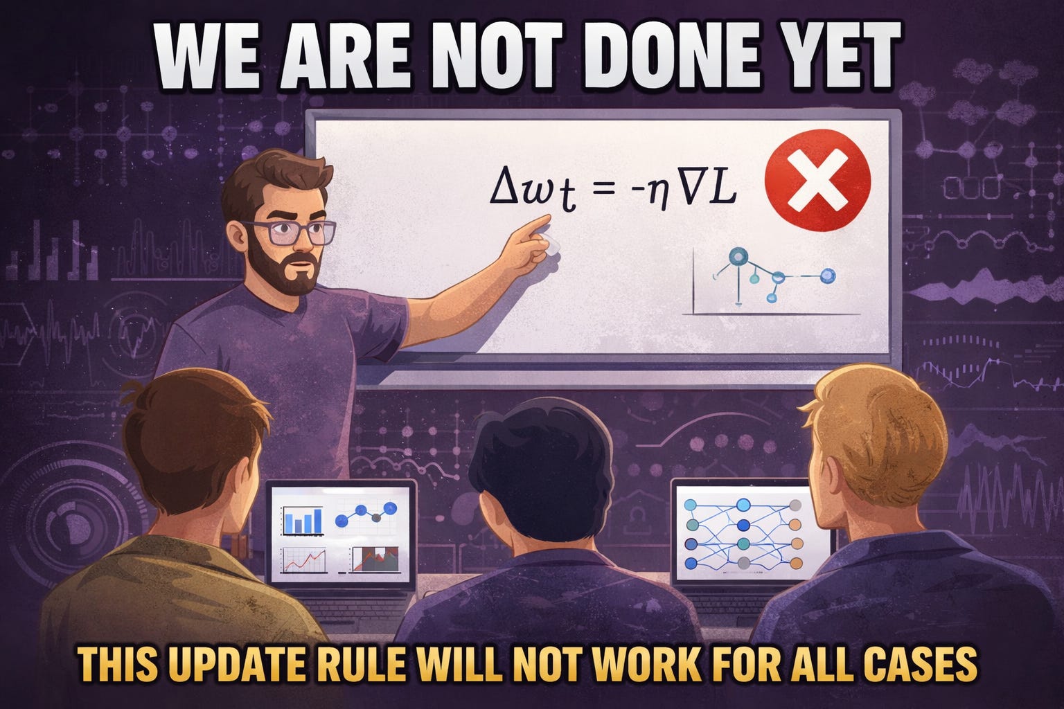
Consider this scenario:

We are at a point where the slope of the mountain is 0, i.e, the gradient is also 0.

This means that we are at a local minima and we are stuck there.

Now, what if there is another minima further down the road which is even below where we are sitting right now? Because of our algorithm, we will never find this minima.

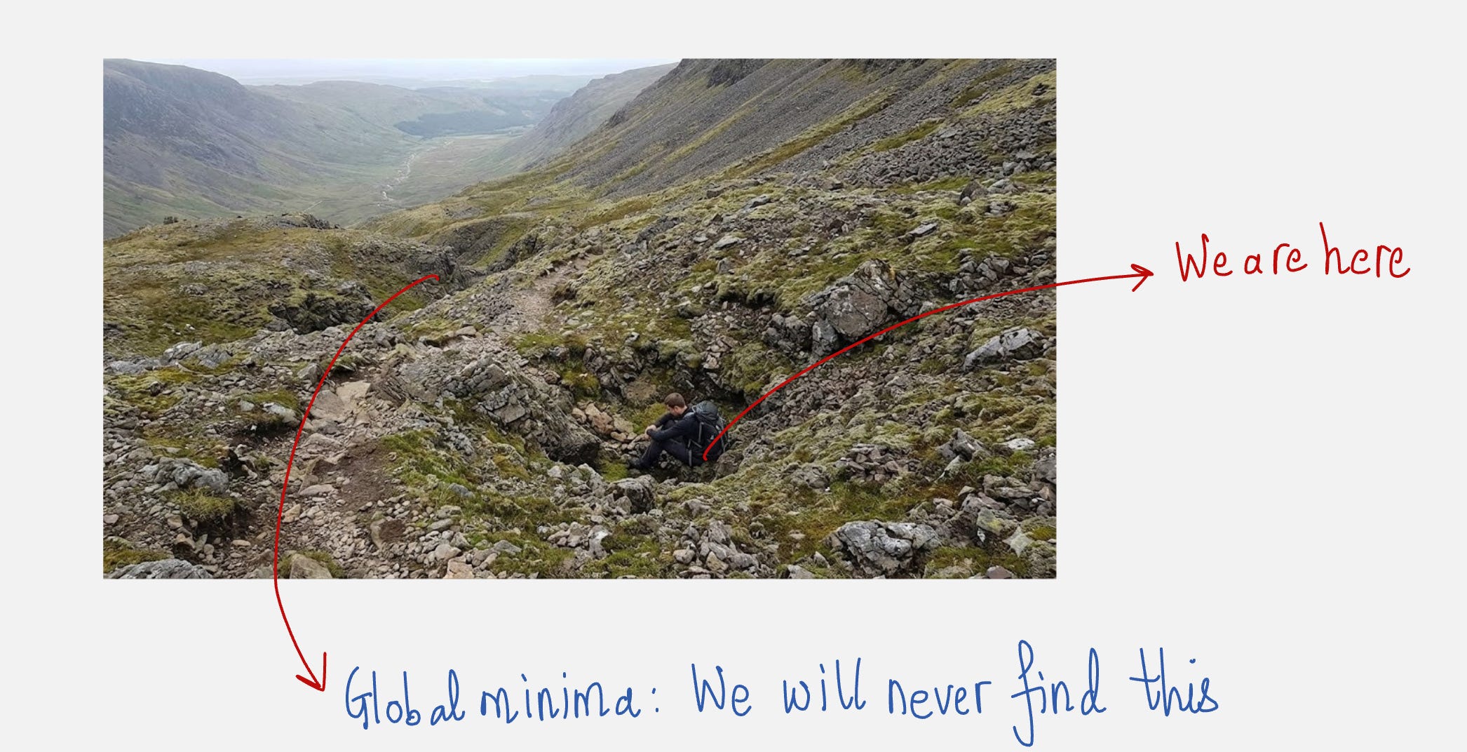
To solve this issue, we need to provide a shake which gives you just enough random energy to kick you out of those small potholes so you can keep moving toward the true bottom of the valley (the Global Minimum).

Remember in the lecture on diffusion, we had discussed about adding noise to the data and we had written a simple expression to add noise which looks as follows:

\(x_{i+1} = x_{i} + \beta \epsilon \)

Refer to the Diffusion article here: https://www.vizuaranewsletter.com/p/what-exactly-are-diffusion-models

The above expression also means that we will sample from a Gaussian distribution with a mean, same as that of x(i), and a standard deviation of beta.

With this same understanding in mind, we will modify our “walking” algorithm as follows:

\(x_{t+1}= x_{t} - \eta \nabla_{x} E_{\phi}(x_{t}) + \sqrt{2\eta}\epsilon_{t}\)

Note that here epsilon represents a random variable which adds an element of stochasticity to the above equation.

This means that even if we are at a local minima where the gradient of the energy function is zero, we will not remain stationary and we will be pulled out of that hole because of that shake provided by the noise term. This will allow us to explore other areas where we might find a global minima.

This equation is also called as Discrete-Time Langevin Update

Now, as we have looked at before, the gradient of the energy function is the negative of the score function. So we can rewrite the above equation as follows:

\(x_{t+1}= x_{t} + \eta s_{\phi}(x) + \sqrt{2\eta}\epsilon_{t}\)

Note that, here we are assuming that we already have a trained score function, and we are understanding how we can sample images from the trained score function using the Discrete-Time Langevin Update.

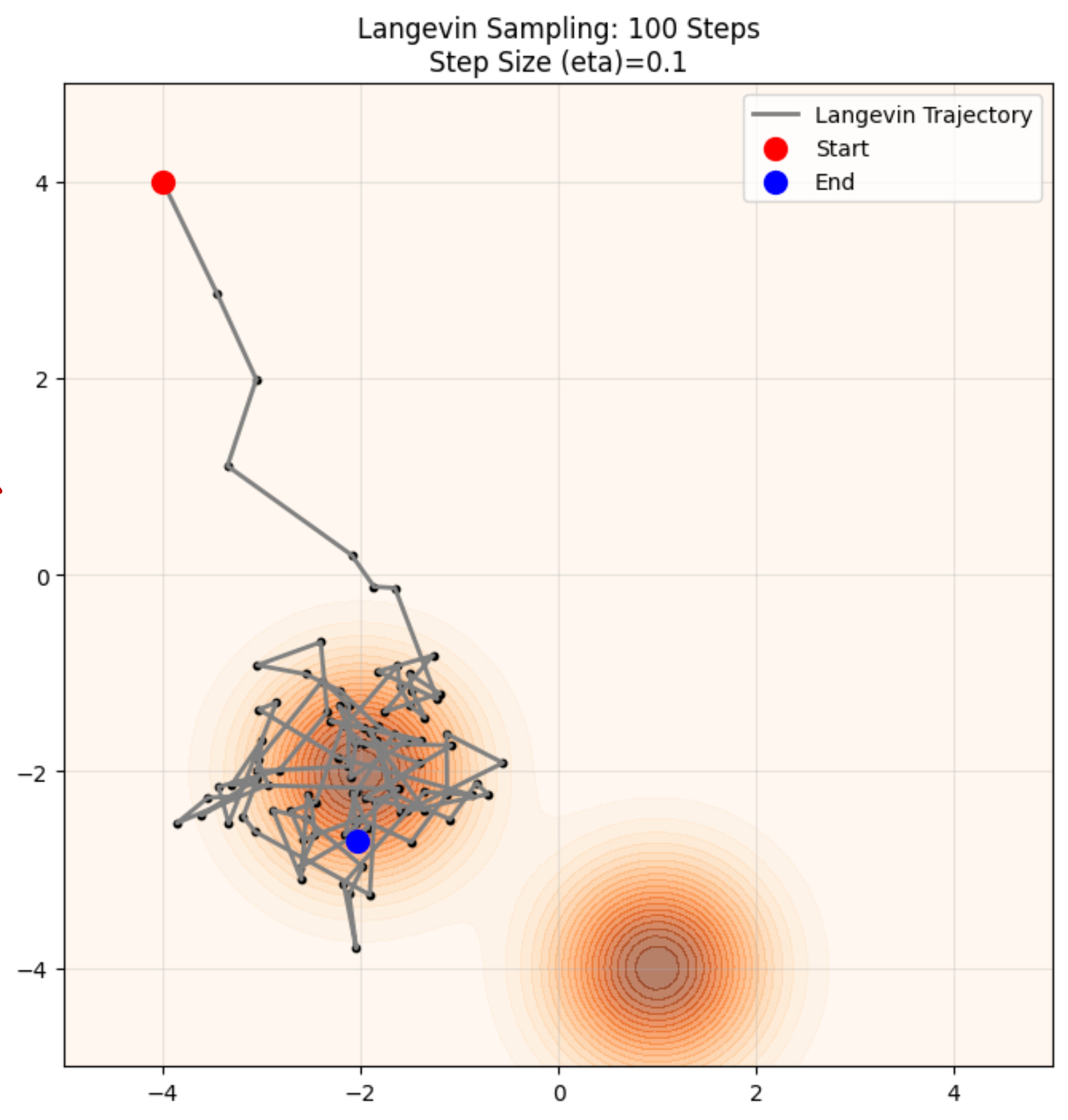
Sampling using the Langevin update tool might visually look as follow

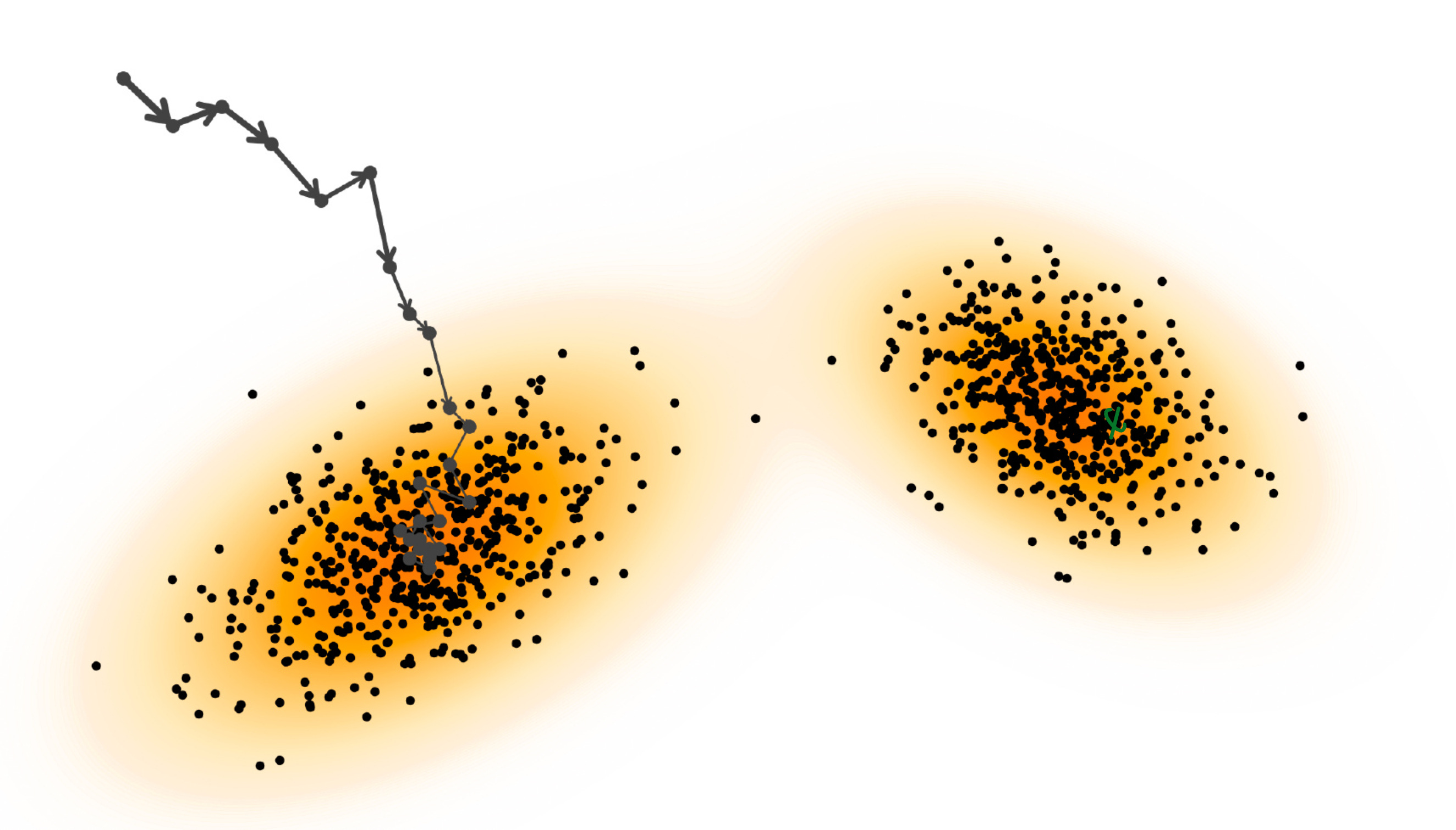
You can see here the zig-zag lines which are the trajectories take from the starting point to the end point. This is exactly because of the stochastic term that we have added in the update rule. It almost looks like a hiker who is drunk and trying to navigate their way in the terrain.

Let us understand this using a practical example. We will use Langevin dynamics to sample from a known probability distribution.

Practical example: Sampling using the Score Function

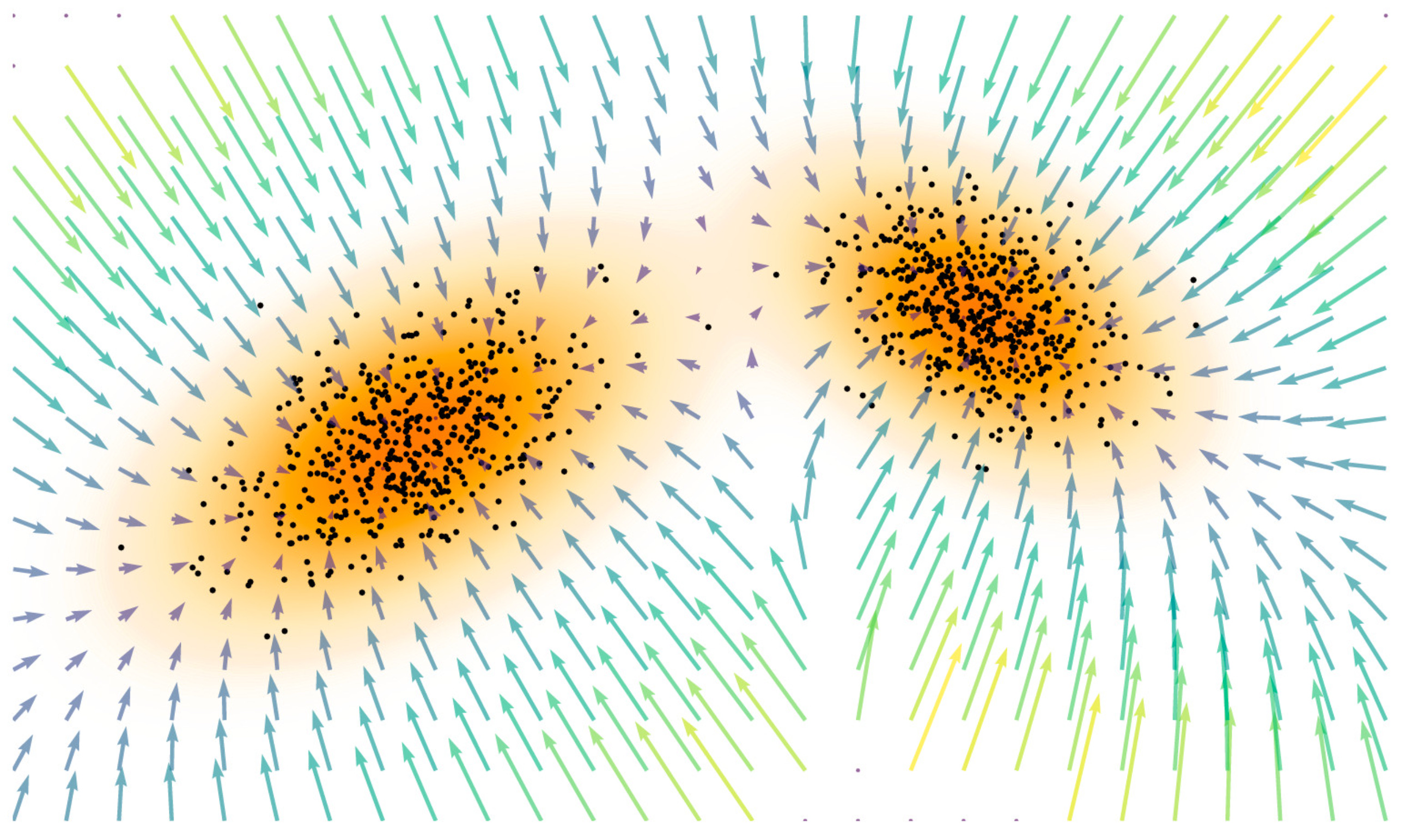
We will use the following the probability distribution as the known probability distribution:

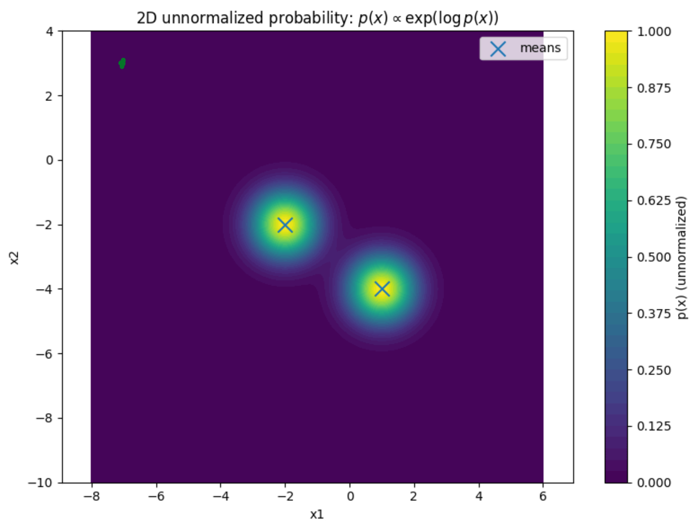
We can see that the distribution has two peaks. There are two regions where the probability of finding the data is the maximum. Then, the probability slowly tapers off as you move away from those peaks.

So, if we start from any point in the grid, our update rule should take us to the areas which appear in yellow color in the contour plot.

This would mean that our update rule has worked successfully, and we have learned to arrive at places where sampling from the probability distribution is the maximum.

Here is the link to the Google Colab Notebook, where we have used the score function in the Langevin update rule to estimate the trajectories.

Google Colab Notebook: Langevin Dynamics - Sampling using a known Score Function

An example trajectory looks as follows:

You can see here that using our update rule, we are reaching towards areas where the probability is the maximum, which is exactly what we want.

So, it looks like we have solved the sampling part. However, this is only 50% of the story.

We are yet to understand how to train our score function so that it matches the true score function as close as possible.

This brings us to Score-based Generative Models.

Score-based Generative Models

The key idea is that since sampling with Langevin dynamics needs only the score, we can learn it directly with a neural network. This shift, from modeling energies to modeling scores, forms the foundation of score-based generative models

Let us look at a sample example:

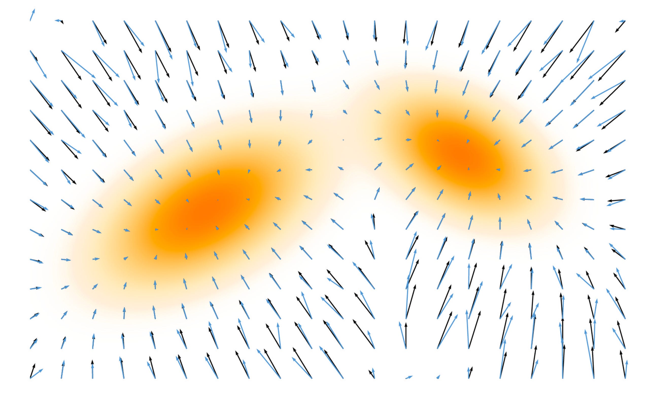
The neural network score (blue) is trained to match the ground truth score (black) using a MSE loss. Both are represented as vector fields.

The true score function is denoted as follows:

\(s(x) = \nabla_{x}\text{log}p_{data}(x)\)

The predicted score function is denoted as follows:

\(s_{\phi}(x) = \nabla_{x}\text{log}p_{\phi}(x)\)

Score matching works by minimizing the mean squared error (MSE) between the true and estimated scores.

The mean squared error loss is given as follows:

\(L_{SM}(\phi) = \frac{1}{2}||s_{\phi}(x) - s(x)||^{2}\)

One of the main problems with this approach is that the true score function is unknown. If we do not know the true probability distribution, then how can we possibly find the gradient of the probability distribution.

Tractable Score Matching:

At first glance, this objective seems infeasible because the true score s(x), which serves as the regression target, is unknown.

Fortunately, Hyvrinen and Dayan (2005) showed that integration by parts yields an equivalent objective that depends only on the model and the data samples, without requiring access to the true score.

This example really highlights the value of research. A paper released 20 years back serves as the backbone of score-based diffusion models. This is truly amazing.

The modified tractable loss function looks as follows:

\(\tilde{L_{SM}}(\phi) = Tr (\nabla_{x}s_{\phi}(x)) + \frac{1}{2}||s_{\phi}(x)||^{2}\)

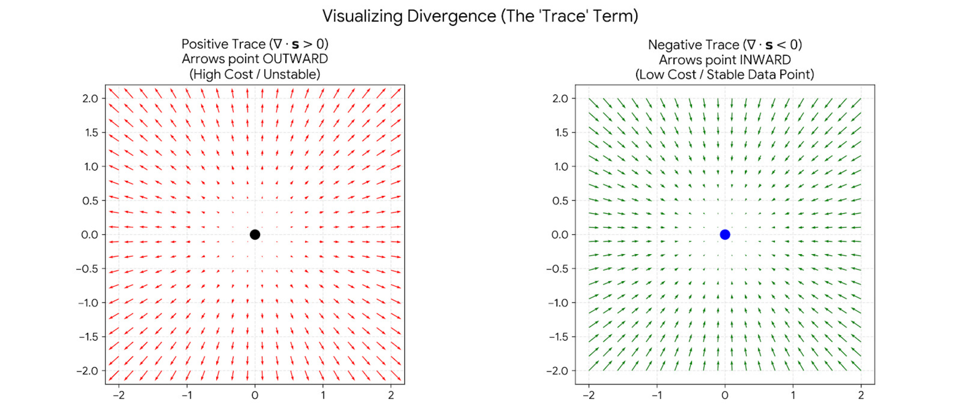
Here, Tr(.) means the trace of the matrix.

Using this objective, we train the score model solely from observed samples, eliminating the need for the true score function.

Let us understand the logic behind both of these terms separately:

Term 1:

This term measures divergence of your arrows. It measures if the arrows are spreading out (exploding) or converging (imploding) at a specific point. Since we are minimizing this loss, we want this value to be extremely negative.

Intuition:

• Positive Trace: Arrows are exploding outward (like a bomb went off).

• Negative Trace: Arrows are sucking inward (like a black hole or a sink drain).

By forcing the trace to be negative at the data points, it forces all the arrows to point INWARD towards the data.

Term 2:

This term measures the length (or strength) of your arrows. It wants the arrows to be as small (short) as possible, ideally zero.

Regions where the probability of the data is high will have more score and contribute more to this term.

This term drives the score to be zero in high probability areas, so that these locations become stationary.

To summarize, the first term makes the high probability areas look as sinks, so that if you take out a compass and want to navigate, you are forced to move inwards towards the high probability areas. Once you are near the high probability areas, you probably don’t want to move too much, and this is achieved through the second term, which makes these points stationary.

Let us look at a practical example where this formulation is used to learn the score function.

Practical Example: Score Matching

In this example, we will solve both parts of the puzzle:

1. We will train the score function

2. We will sample from it

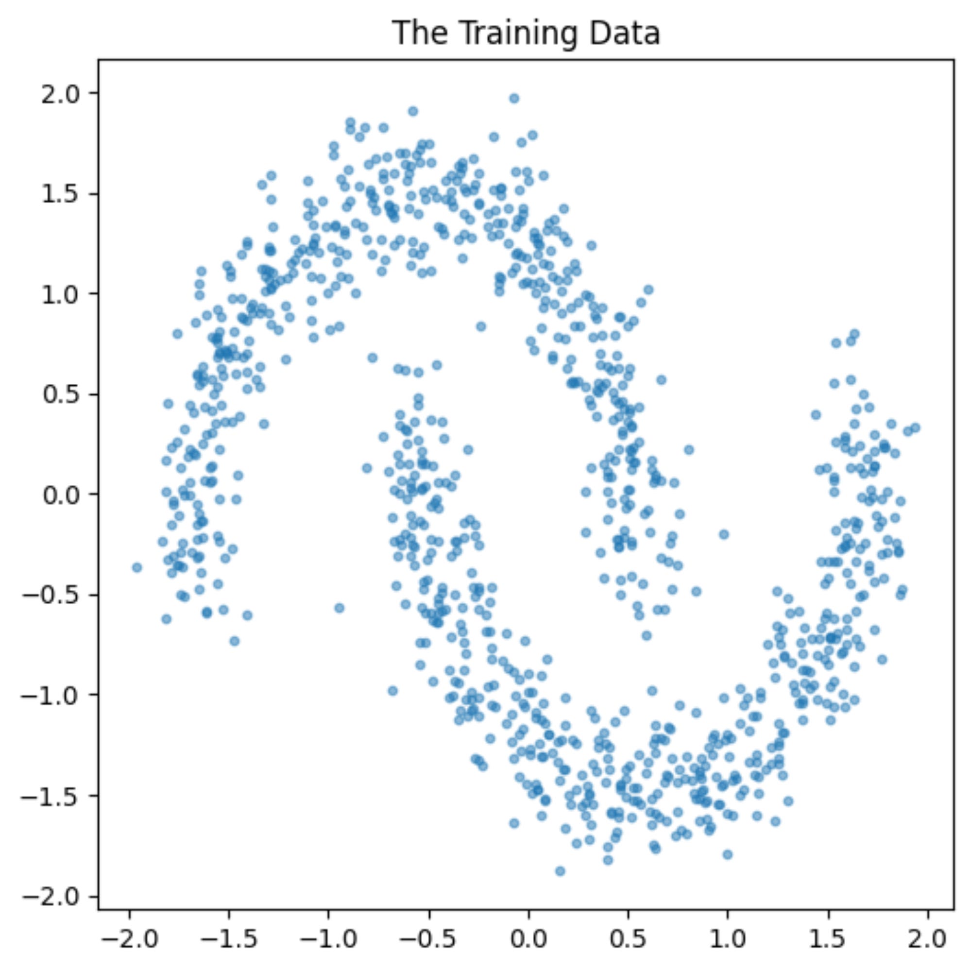
We will learn to predict the score function for this data.

Here is the link to the Google Colab notebook which uses the tractable score matching loss formulation to solve this problem:

Google Colab Notebook - Using the tractable Score Matching Loss Formulation

This is final learnt score function which we get:

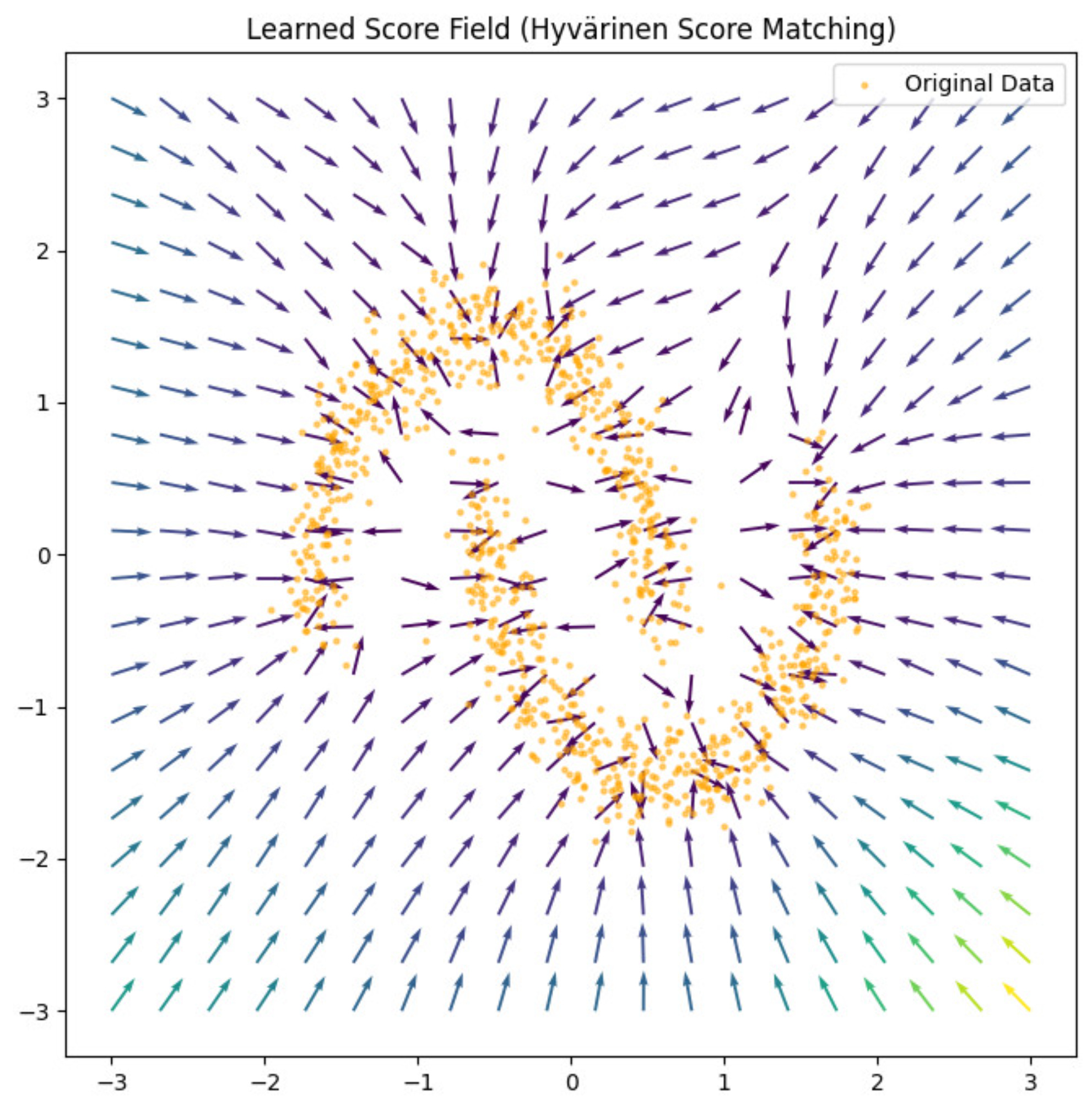
From the above image, we can see that how this score function acts like a compass which points us to the region where the data is located.

We can also see some regions like sinks which are created near the data which pull you inside and so you are close to those regions.

So, it looks like we have managed to train our score function properly :)

Once this score field is learned, we can also sample from it using Langevin Dynamics, exactly as we have learned before:

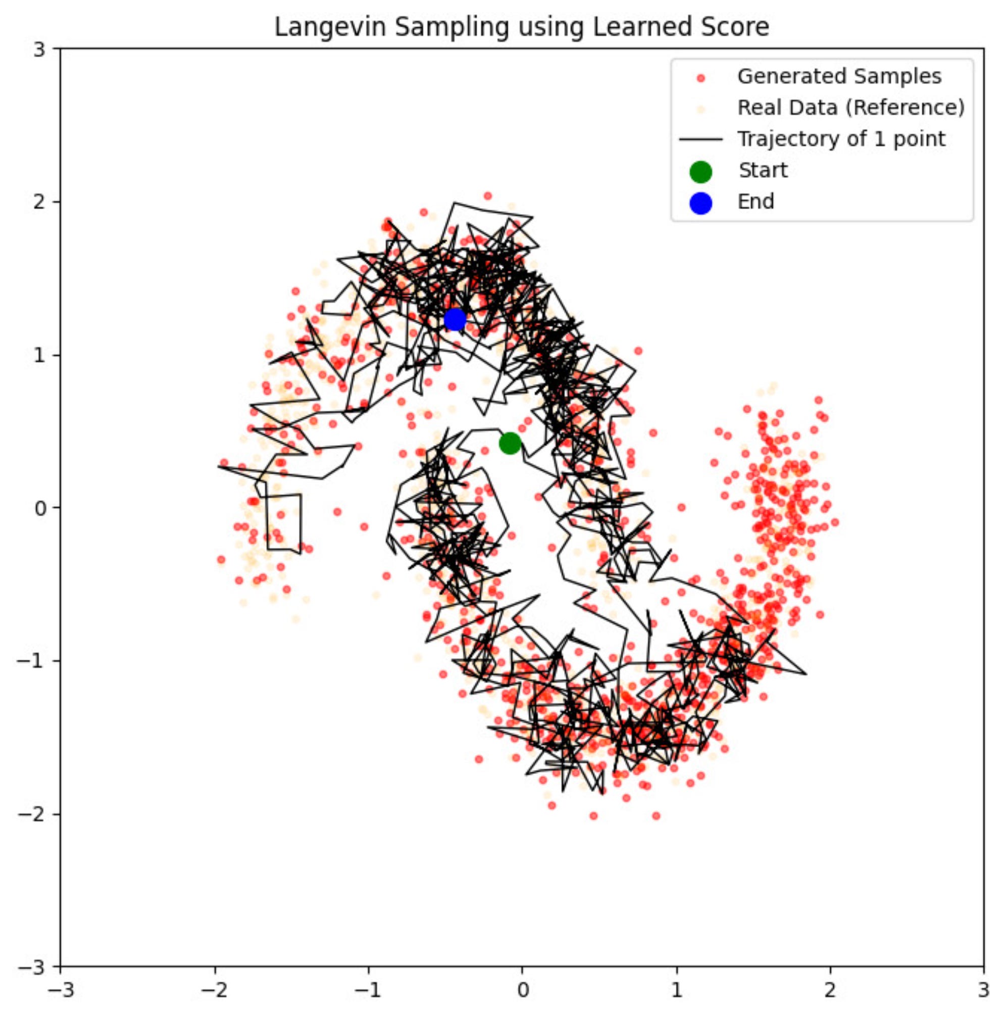
We start from the “green point” and end in the “blue point”. This trajectory is calculated using the Langevin Dynamics update rule which we looked at before.

Our “drunk hiker” does quite well in ending up close to the area where the probability density of the data is high :)

That’s it! This was the score matching formulation as one of techniques in Deep Generative Modeling.

It is very interesting to note that these two tracks of diffusion models and score-based models appear very distinct, but they converge very nicely together. We can understand both of them using a single unified framework

We will look at this in the next chapter, where we will examine the foundational role of the score function in modern diffusion models.

Initially introduced to enable efficient training of EBMs, the score function has evolved into a central component of a new generation of generative models.

Here is the link to the original paper which introduced the tractable Score Matching formulation): https://arxiv.org/abs/2006.11239

For further reading, please refer to the book: The Principles of Diffusion Models From Origins to Advances (https://arxiv.org/abs/2510.21890) [Pages 56-68]

If you like this content, please check out our bootcamps on the following topics:

Modern Robot Learning: https://robotlearningbootcamp.vizuara.ai/

GenAI: https://flyvidesh.online/gen-ai-professional-bootcamp

RL: https://rlresearcherbootcamp.vizuara.ai/

SciML: https://flyvidesh.online/ml-bootcamp

ML-DL: https://flyvidesh.online/ml-dl-bootcamp

CV: https://cvresearchbootcamp.vizuara.ai/