
How to Combine Physics and Machine Learning?
A Complete SciML Project Walkthrough


Can a neural network learn the hidden structure of the physical world?
More importantly, can it work with the known laws of nature instead of replacing them?
In this article, I will walk you through a complete Scientific Machine Learning (SciML) project - step by step - where we blend the predictive power of ML with the interpretability of physics-based models.
Whether you are an economist, physicist, engineer, or researcher from any field, this project will show you how to bring ML into your work without throwing away decades of domain knowledge.
Let us get started.
The problem: We know some laws, but not all
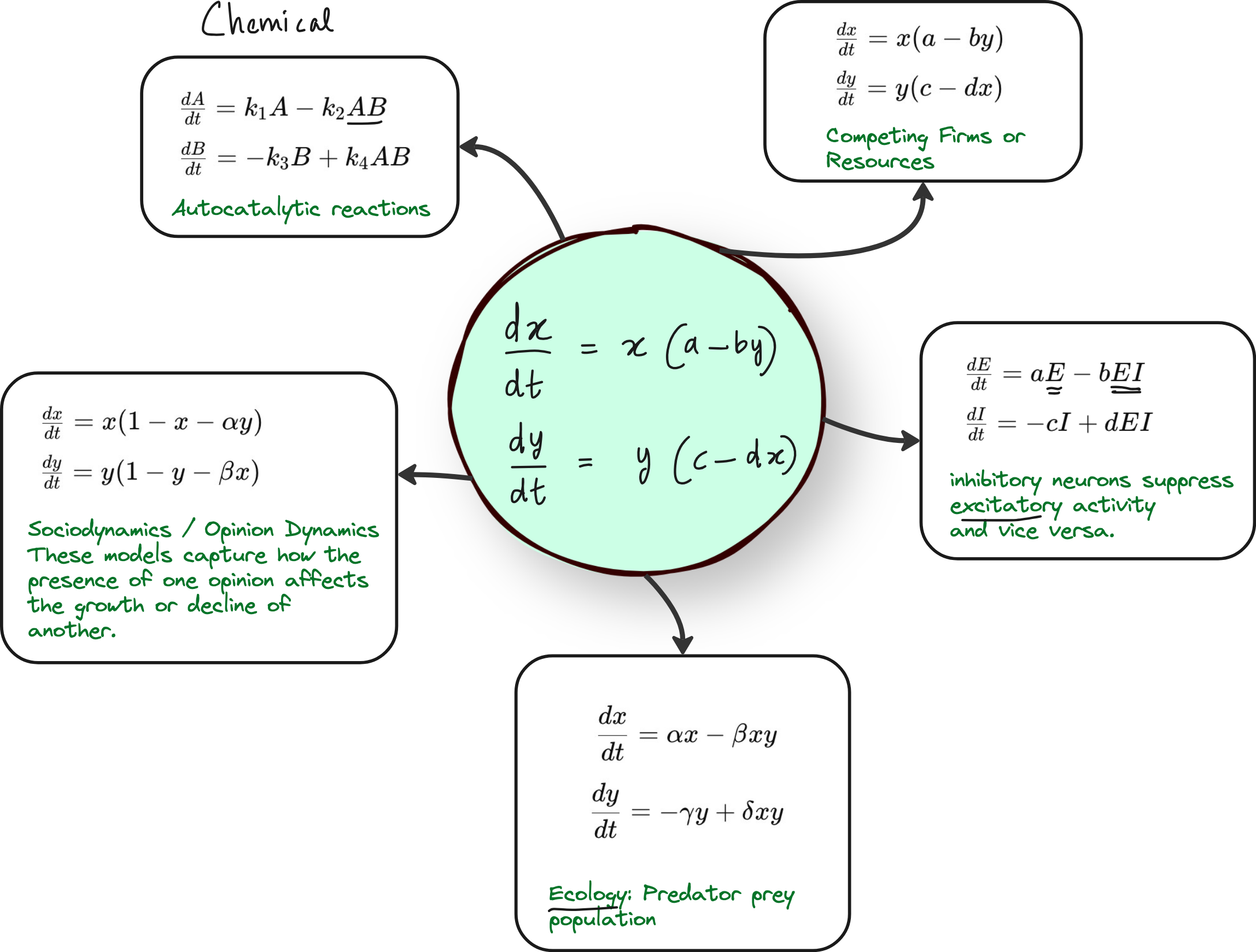
Most scientific systems can be modeled using differential equations.
For example:
In ecology: predator-prey dynamics
In neuroscience: excitatory and inhibitory neurons
In economics: firms competing for resources
All of these can be described using systems of ordinary differential equations (ODEs).
But in practice, some terms in the equation are missing or unknown. That is where pure mechanistic modeling breaks down.
And that is exactly where Scientific Machine Learning steps in.
Step 1: Start with a familiar ODE - The Lotka-Volterra system
We use the well-known Lotka-Volterra equations - a class of nonlinear differential equations.
While they originated in ecological modeling (e.g., predator-prey systems), the same mathematical framework appears across many other domains due to its general structure of nonlinear interaction between components.
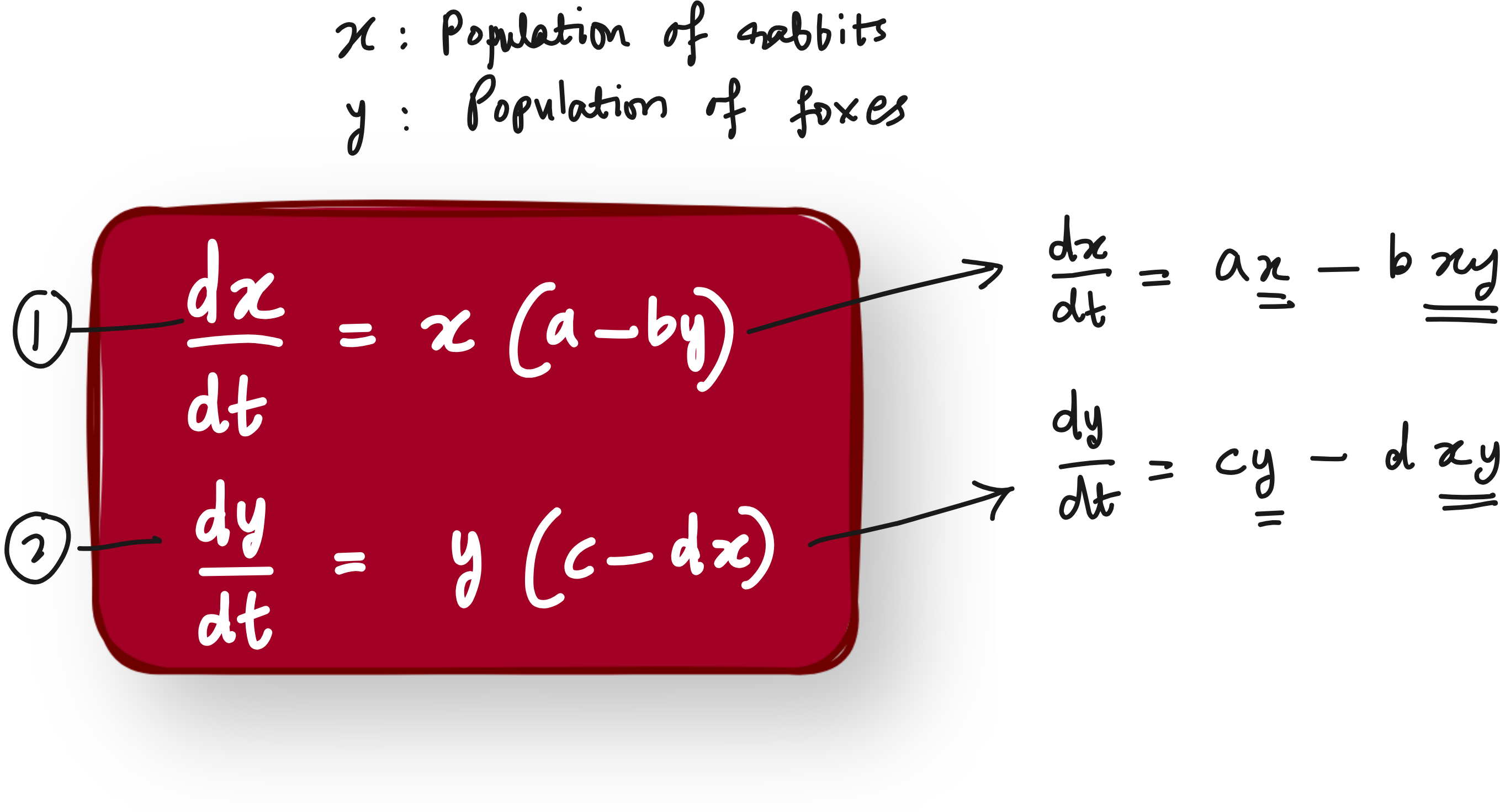
Lotka-Volterra system of equations can be adopted to many fields, not just for the prey-predator model.
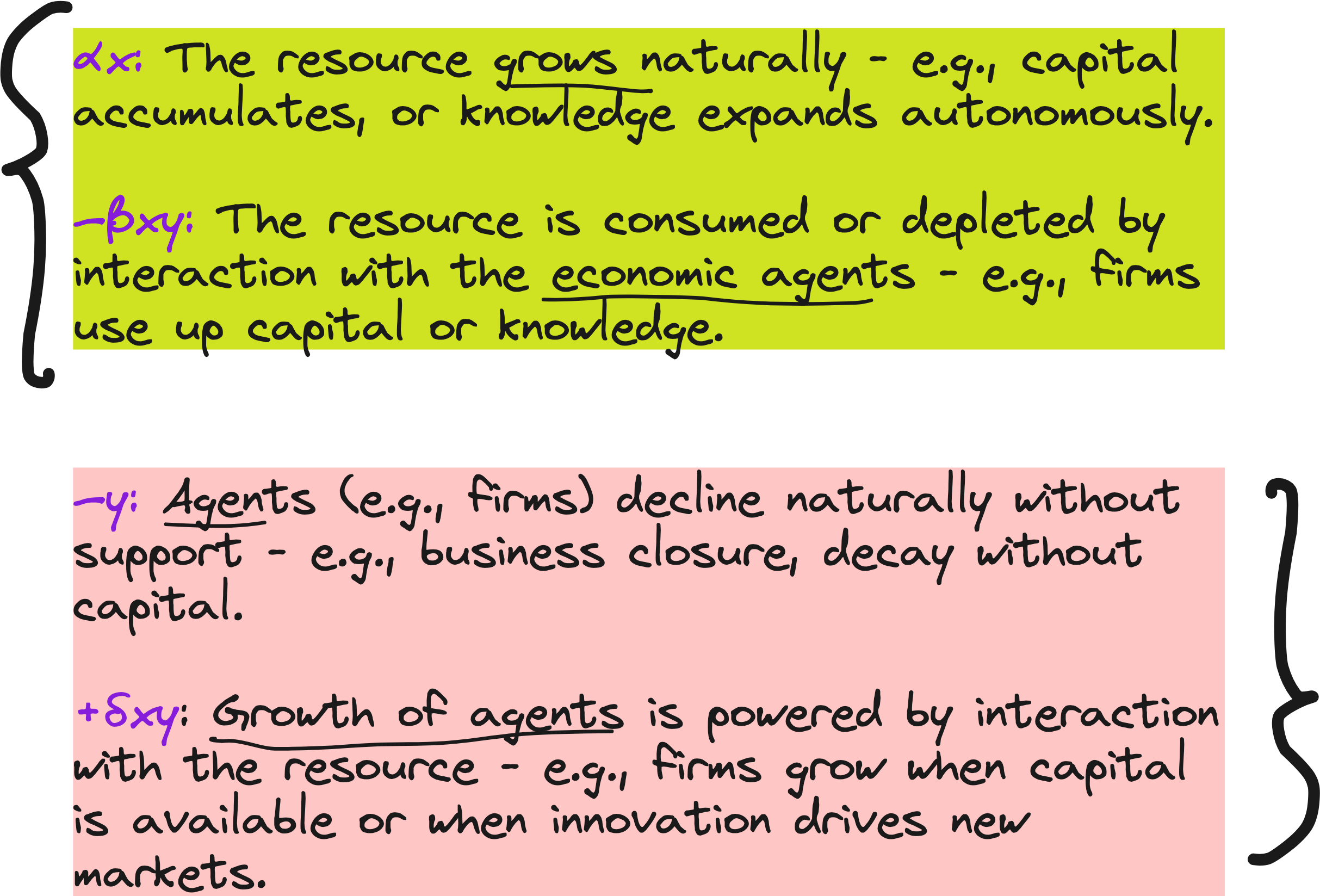
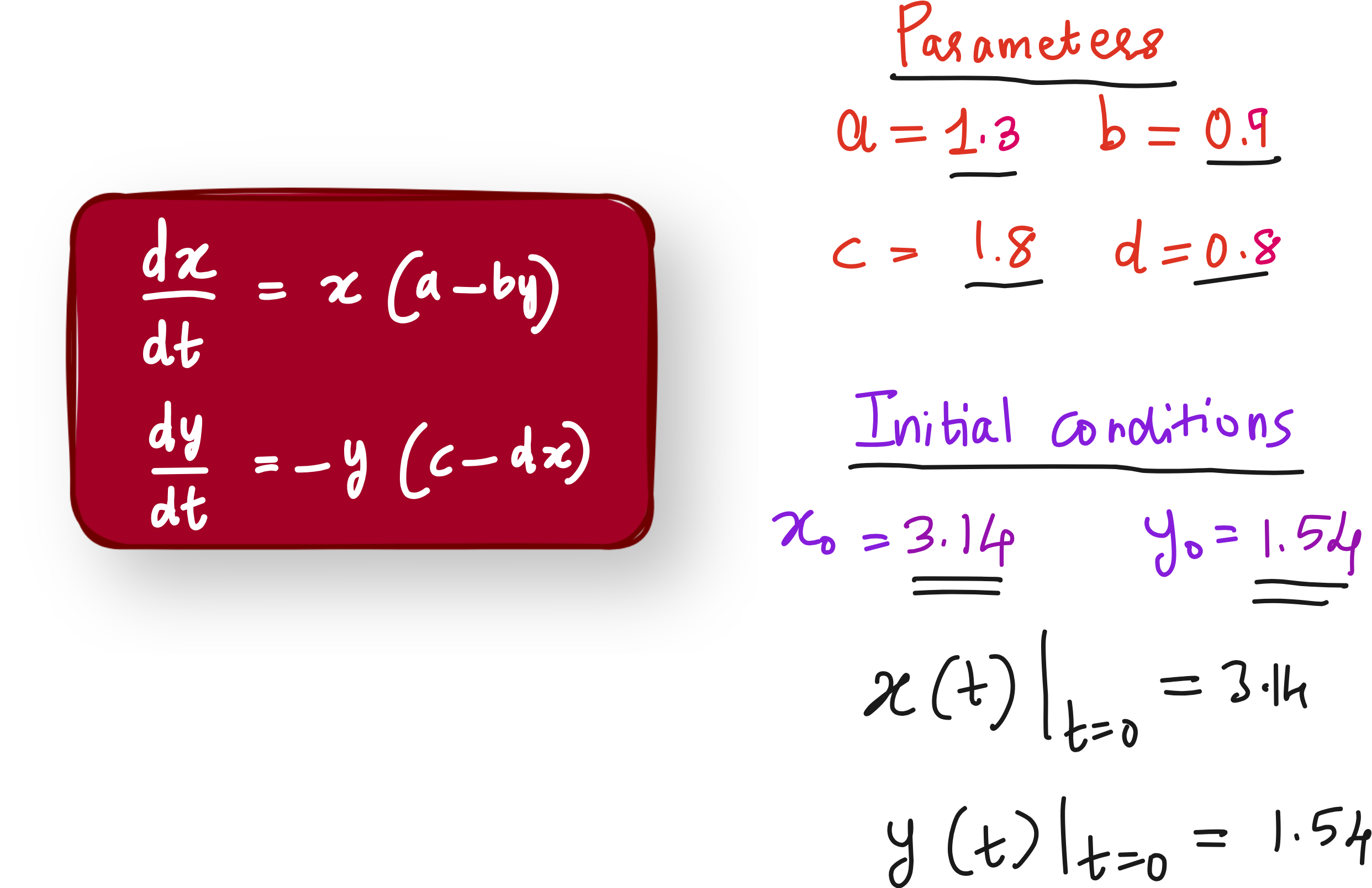
We slightly adapt this to model an economic system:
x(t)represents available capital or resourcesy(t)represents the number of firms or economic agents
The interaction between capital and firm growth is modeled as:
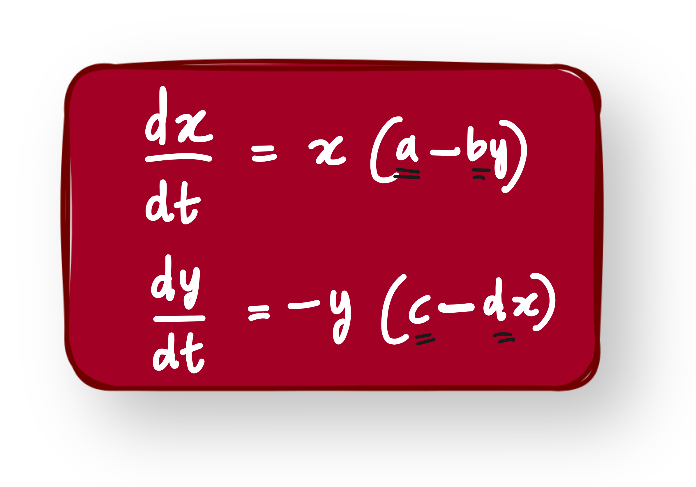
This already gives us useful dynamics: boom and bust cycles, saturation effects, etc.
But now we assume we do not know the exact form of the interaction terms bxy and dxy. Could they be nonlinear? Could they be something else entirely?
Step 2: Replace unknown terms with a Neural Network
This is where Universal Differential Equations (UDEs) come in.
Instead of guessing the form of the interaction terms, we replace them with a neural network:
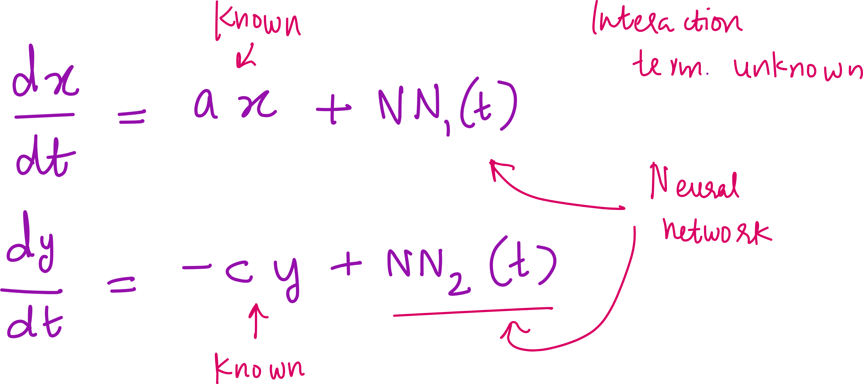
We keep the known linear terms intact (like
ax,-cy)We let the neural network approximate the unknown parts
This hybrid model has the interpretability of equations and the flexibility of ML. It is the best of both worlds.
We build this using Julia, the perfect language for scientific computing. Libraries like DifferentialEquations.jl, Lux.jl, and Optimization.jl allow tight integration of ODE solvers and neural nets.
Step 3: Let us build the ground-truth data
Since we don’t have readily available experimental data, we can construct the ground truth data by solving the original Lotka-Volterra ODE equation system with initial conditions and parameter values. We use Julia’s ODE solver for this.
Step 4: Train the Neural Network on simulated Data
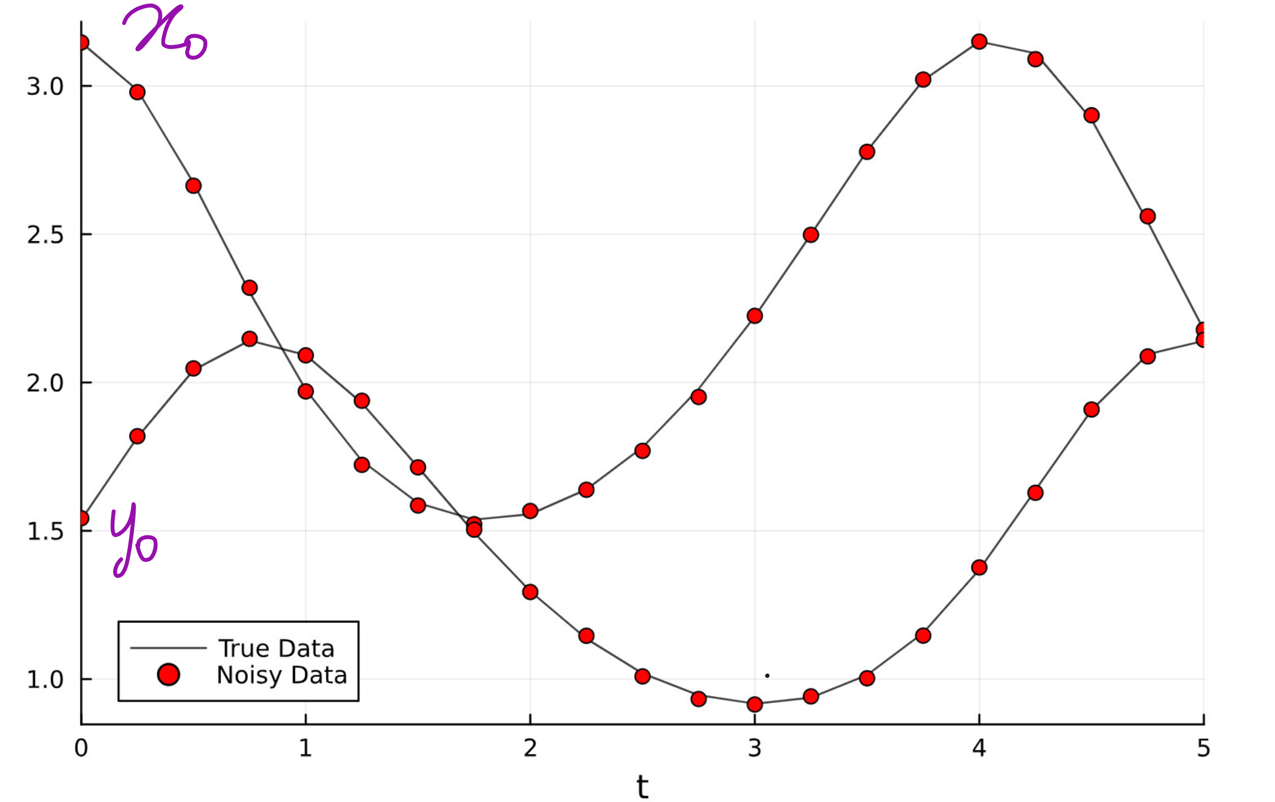
Since we do not have real-world data for this exact system, we simulate the ground truth using the full Lotka-Volterra model with known parameters.
We add small Gaussian noise to make it realistic.
Then we train the UDE to match this data.
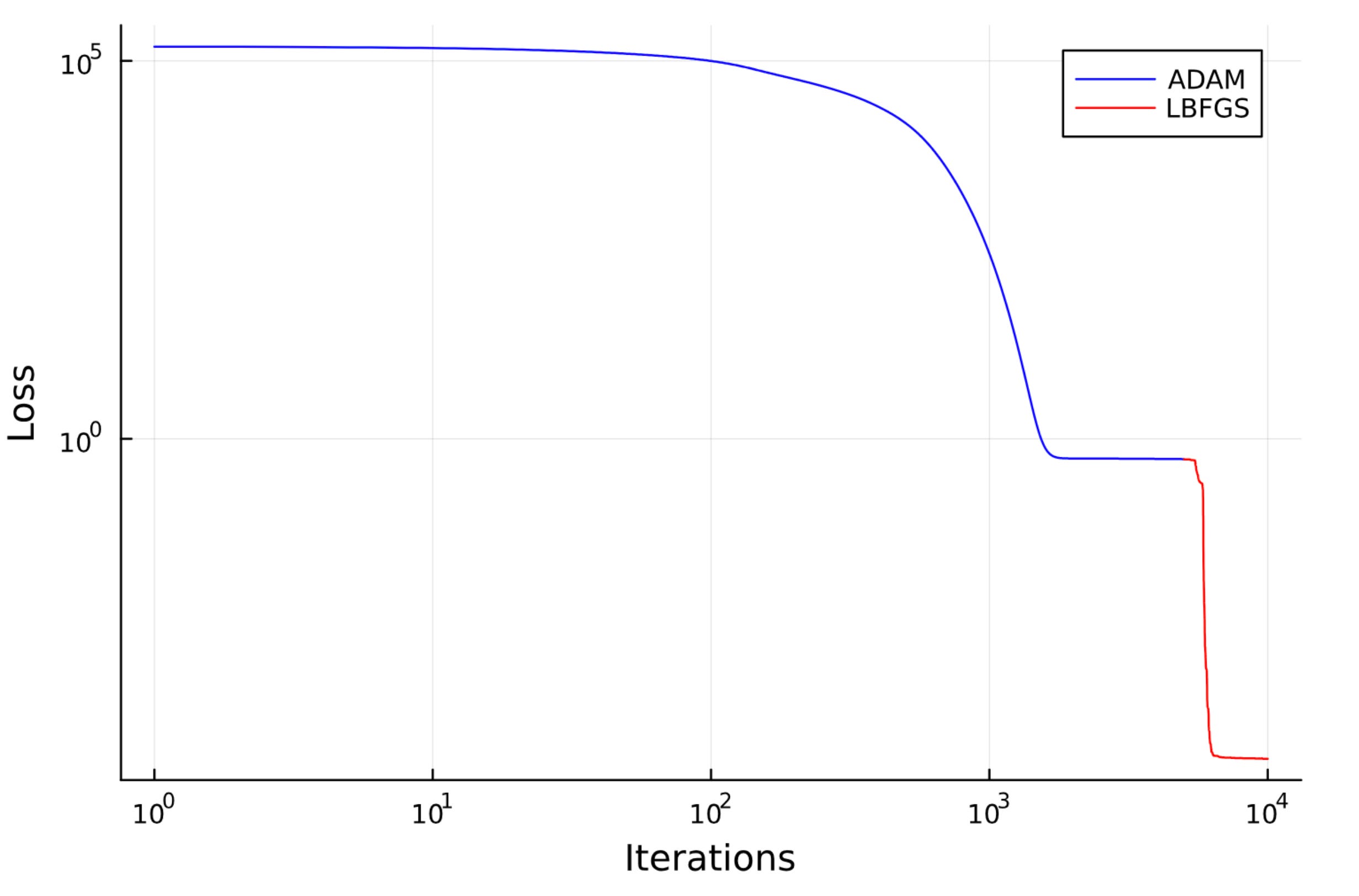
Optimizer Strategy:
First 5,000 iterations with Adam optimizer
Next 10,000 iterations with LBFGS (great for final convergence)
This two-stage strategy ensures fast convergence and a low final loss.
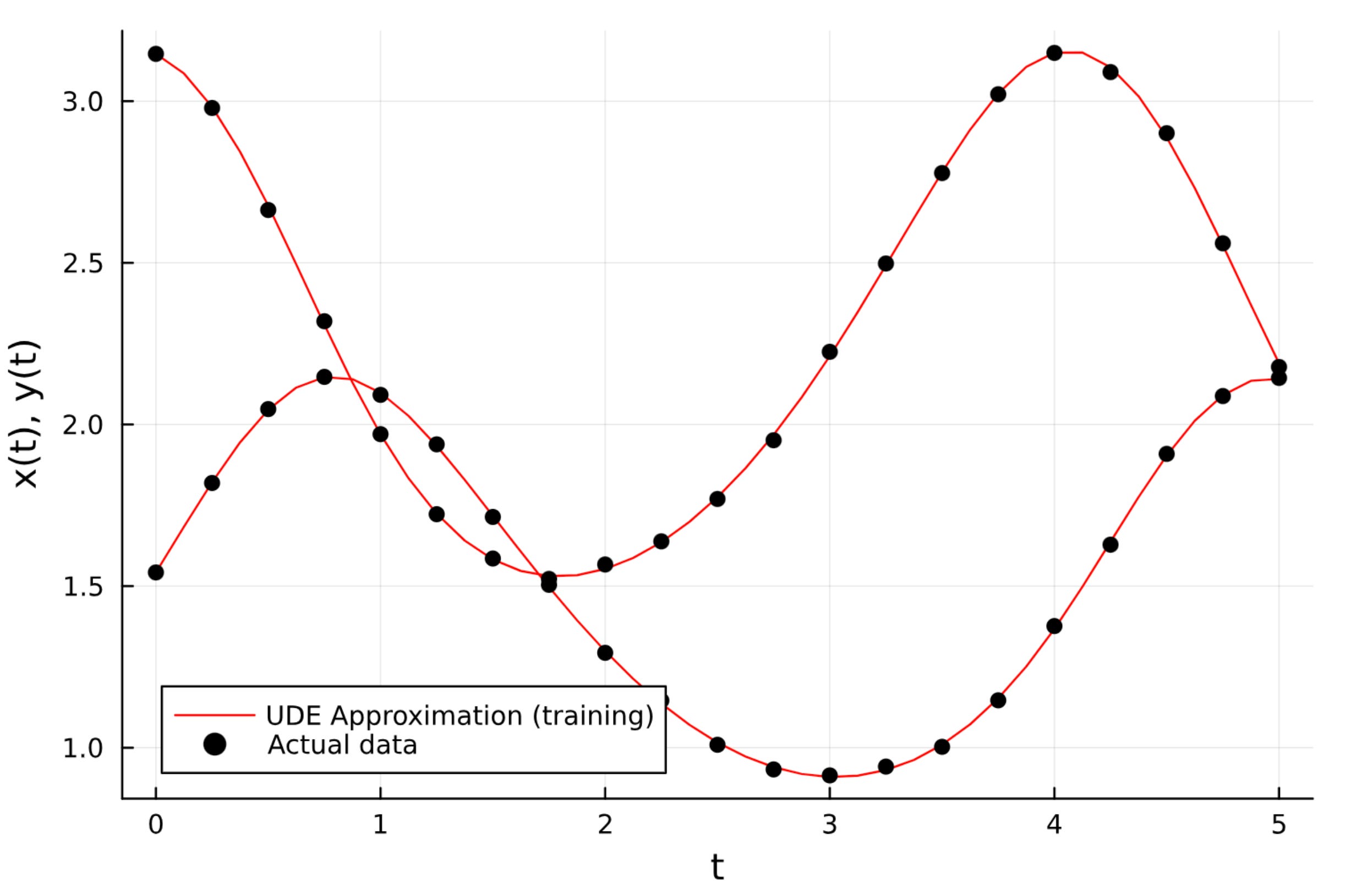
Eventually, we reach a loss of 5 × 10⁻⁵, showing that the neural network has learned to approximate the unknown interaction terms very well.
Our UDE predictions perfectly match the noisy ground truth data as shown in the plot below.
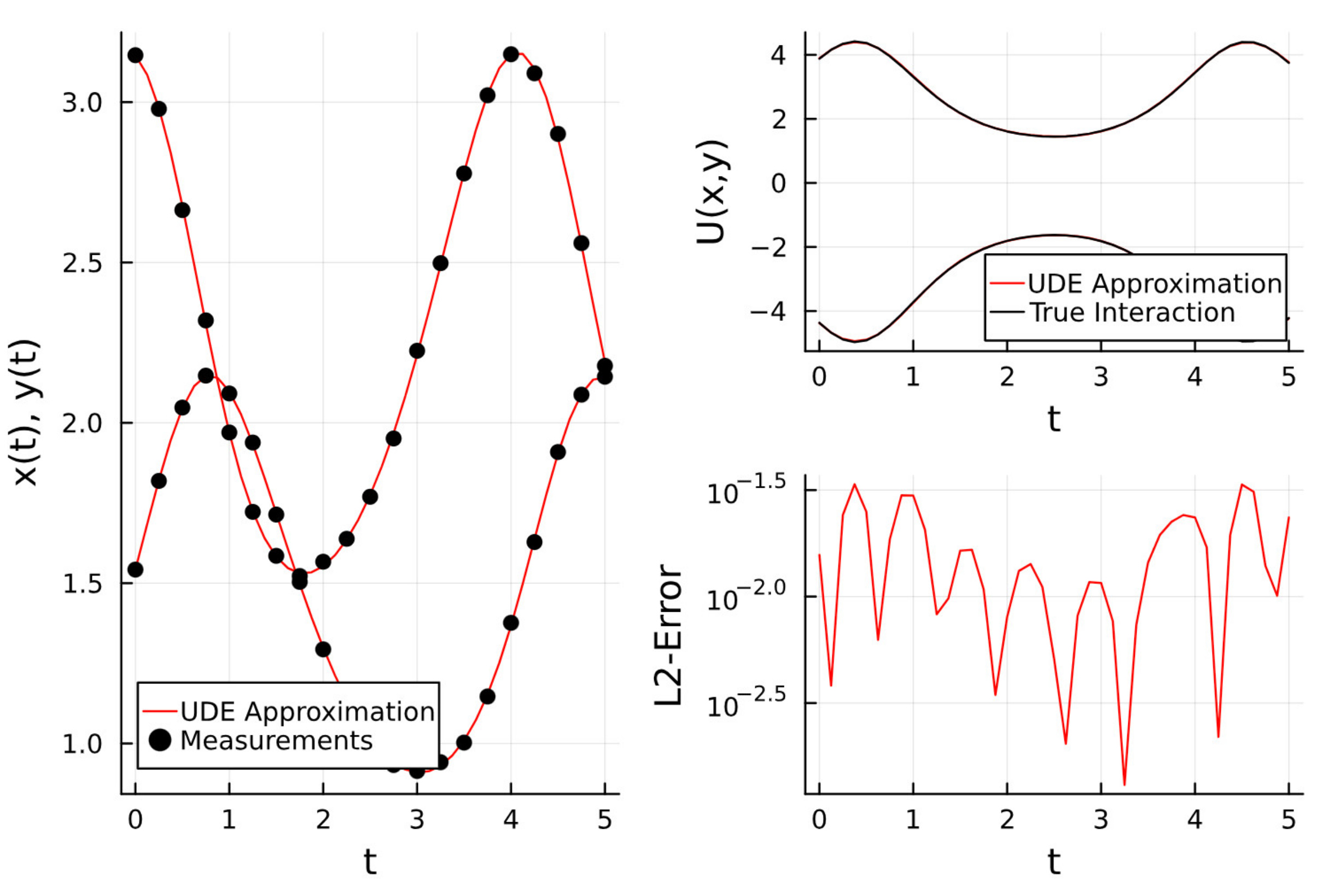
We can also plot the loss as well as the expected and predicted values of the interaction terms. The match is perfect as shown in the plots below.
Step 5: Forecast beyond observed time
Once the model is trained, we use it for forecasting.
We extend the time range beyond the training window and observe how well the model performs.
Because the UDE model still relies on known physics, it extrapolates much better than pure ML models.
In traditional ML, you need 80% of your data for training. In SciML, you can get great forecasting with just 20% of the data, because the model already understands the system's structure.
Step 6: Recover the governing equation via symbolic regression
This is where things get even more interesting.
What if we could extract the actual mathematical form of the interaction terms the neural network learned?
We do this using symbolic regression.
We feed the predicted interaction terms into a regression engine and define a basis function library (e.g., 1, x, y, xy, x^2, y^2, etc.).
We use a library of 15 basis function as shown below.
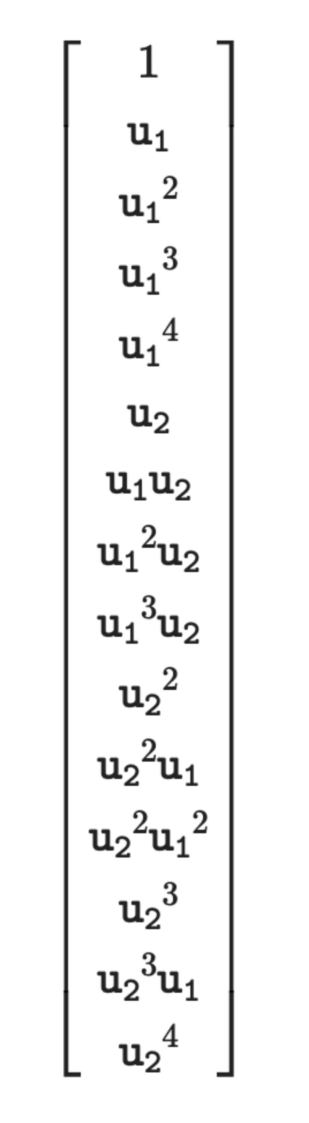
Here u1 corresponds to x and u2 corresponds to y.
Using the basis functions we construct design matrix. To read a bit more in detail, check out this article:
Can AI discover the laws of nature from data alone?

There is something deeply human about discovering a law.
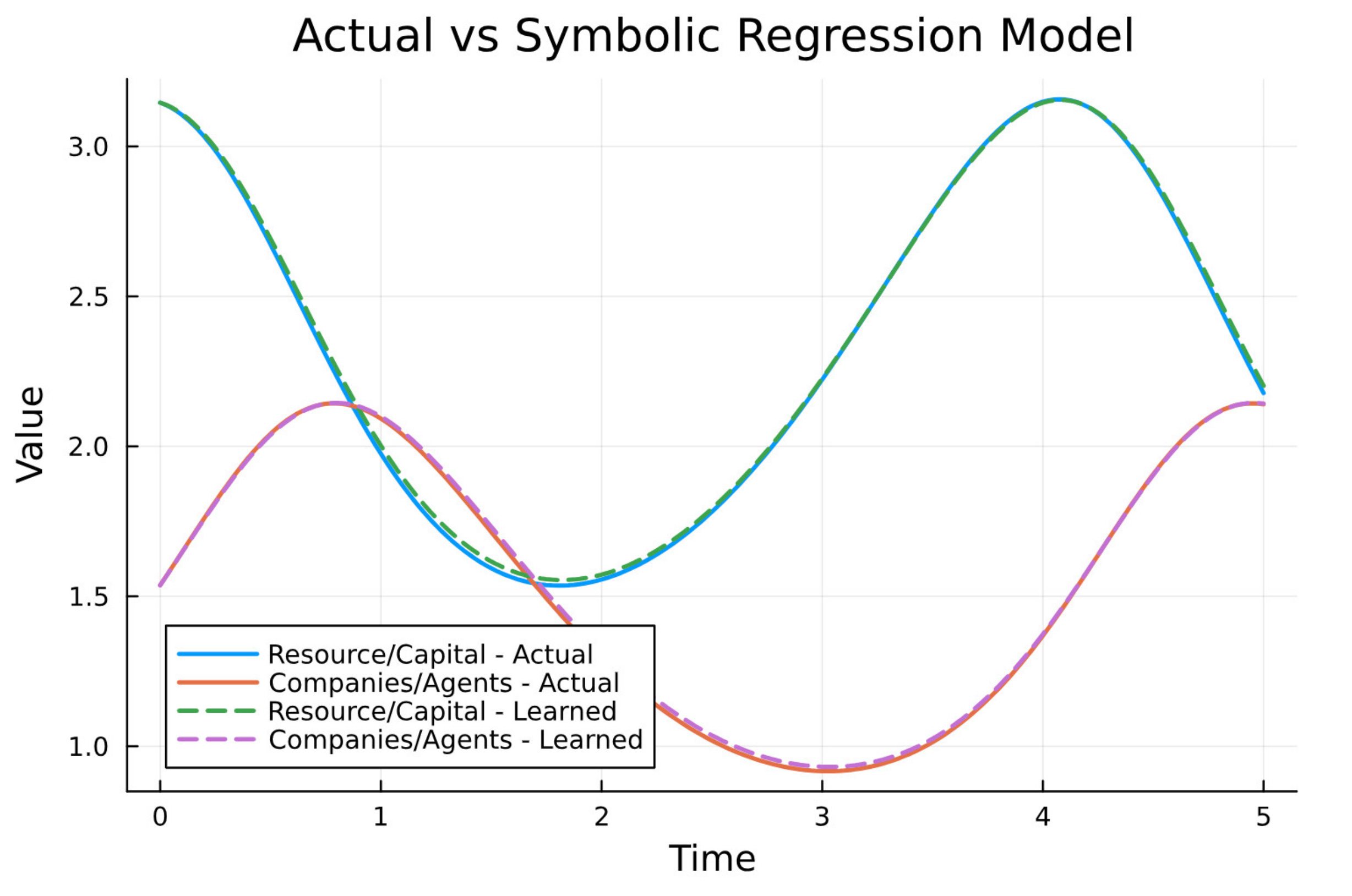
The result?
NN1(x,y)≈−0.88xy
NN2(x,y)≈+0.75xy
Exactly what we had in our original Lotka-Volterra model.
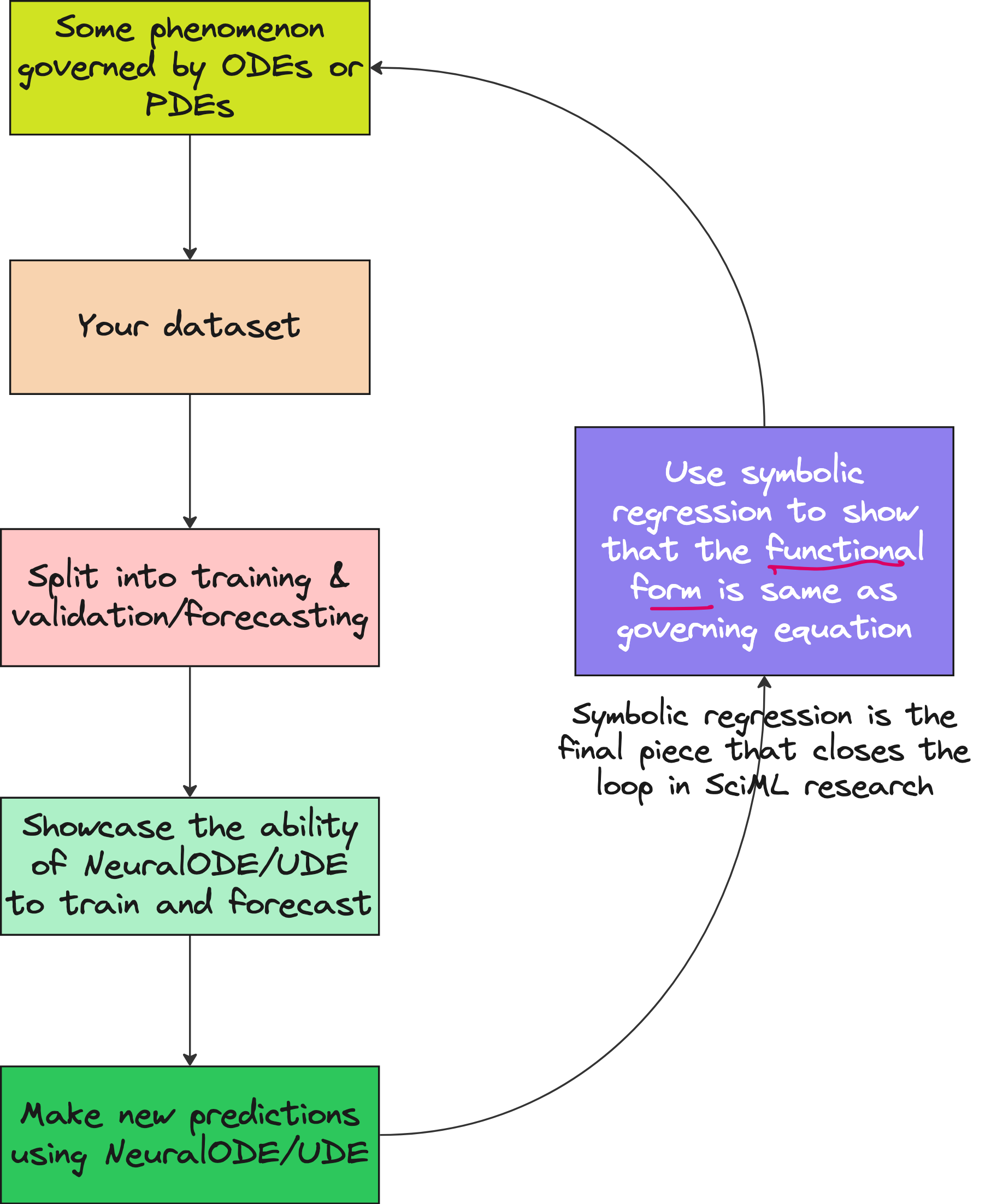
This closes the loop.
We went from:
Unknown system →
Partial ODE + Neural Network →
Predictions →
Symbolic recovery of the actual governing law
Why This Matters
In physics, Newton did not use data to train a model.
He derived the law from observations.
With SciML, we are doing something similar.
We use data to re-discover the laws of nature.
You can apply this same workflow to:
Epidemiology
Astrophysics
Neuroscience
Materials science
Economics
Battery degradation
Any domain with partially known dynamics
Resources
🧠 Full Code File:
https://drive.google.com/file/d/1DJhIgulv6878N68_8ECwuX--rGxpfn5d/view?usp=sharing
🎥 Full Lecture Video:
Want to do real SciML research?
Check out our bootcamp for students, engineers, and researchers:
https://flyvidesh.online/ml-bootcamp/