Can AI discover the laws of nature from data alone?

Introduction to Symbolic Regression

There is something deeply human about discovering a law.

A handful of scattered observations. A pattern you cannot quite place. Then, the sudden click of a clean equation that explains it all. That feeling is what drives science. And it is exactly what symbolic regression replicates - but through a machine.

Not just to fit curves.

Not just to minimize error.

But to actually rediscover the structure that generated the data in the first place.

This is the story of how I taught a machine to rediscover a simple quadratic equation. What began as a five-point dataset evolved into a fascinating journey through sparsity, symbolic modeling, and the nature of discovery itself.

Forget the formula

Let us start with a simple quadratic equation:

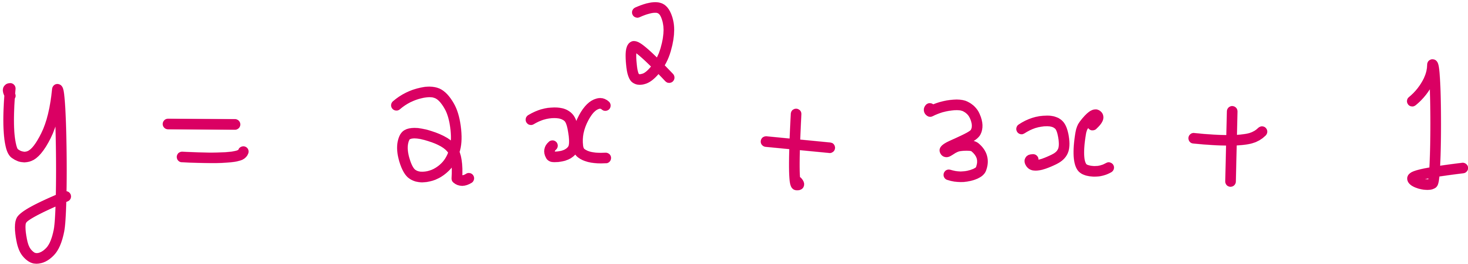
Now forget it. Wipe it from your memory.

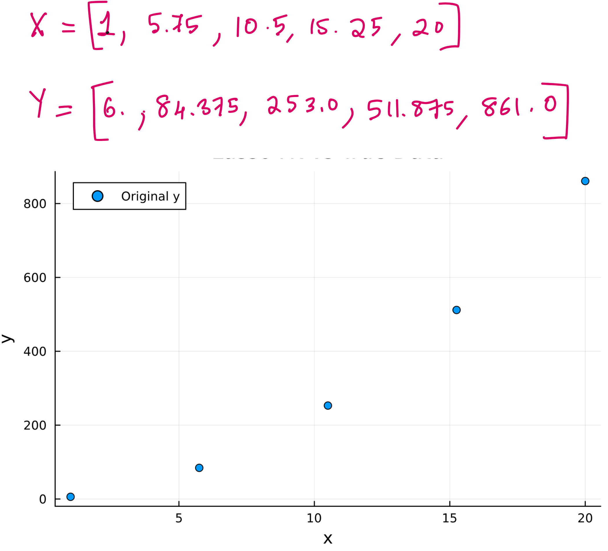
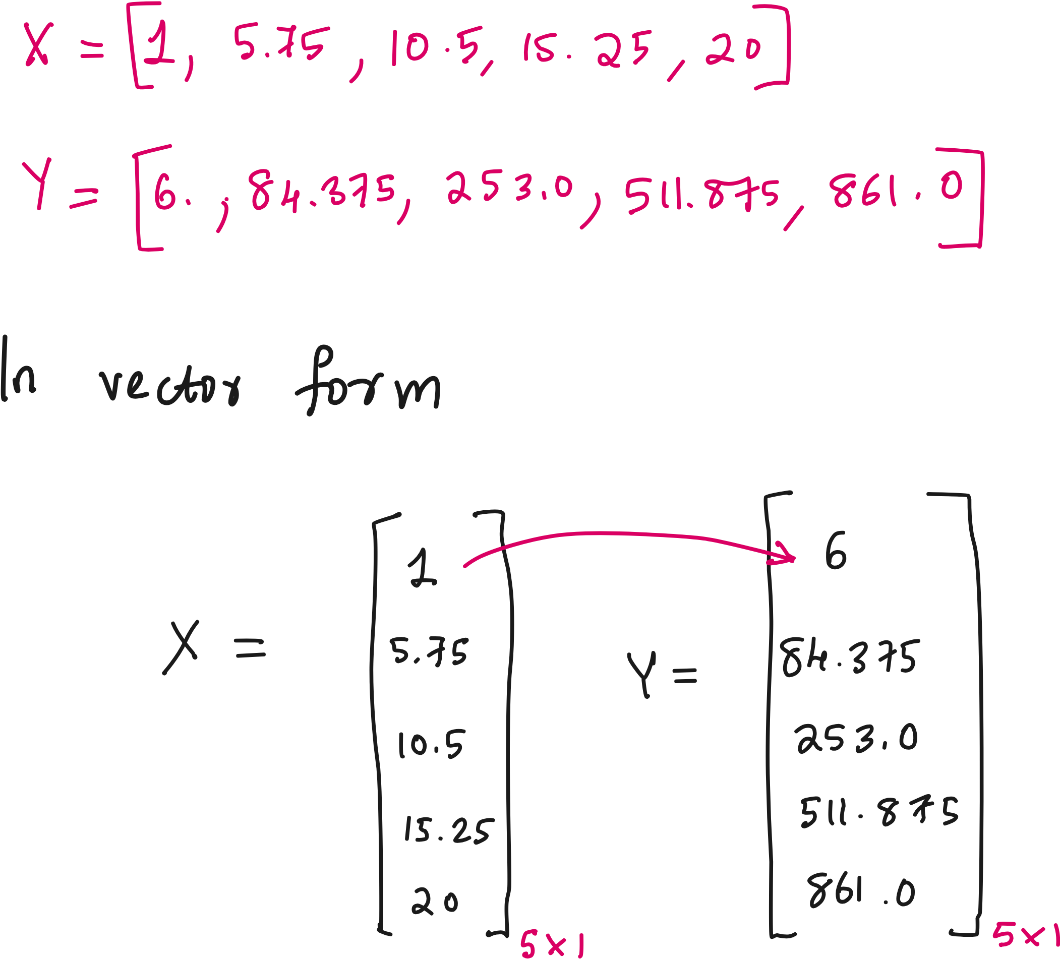
You are handed five input-output pairs. The inputs are five values of x, and the outputs are the corresponding values of y. But you are not told the equation that links them.

Your task is simple.

Find the rule.

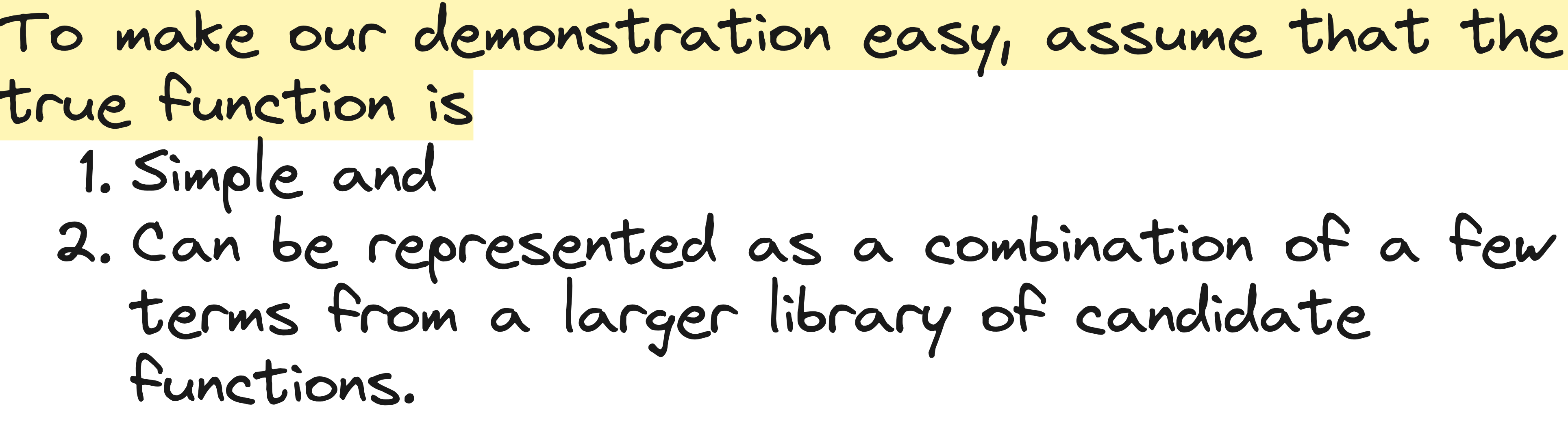
Not by assuming a polynomial of a certain degree. Not by curve-fitting with black-box tools. But by allowing the machine to discover the functional form itself - from scratch.

This is symbolic regression.

Beyond regression, toward reasoning

In regular regression, you define the structure. You might decide that y depends on x and x^2, and let the model solve for the coefficients. But what if you do not know the structure? What if you want the model to figure it out?

That is the leap symbolic regression takes.

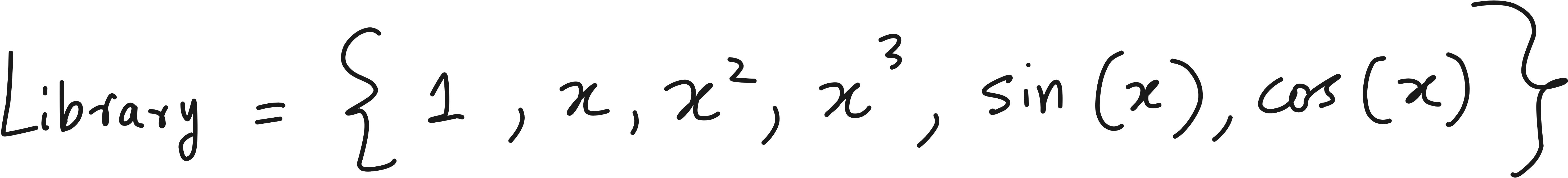
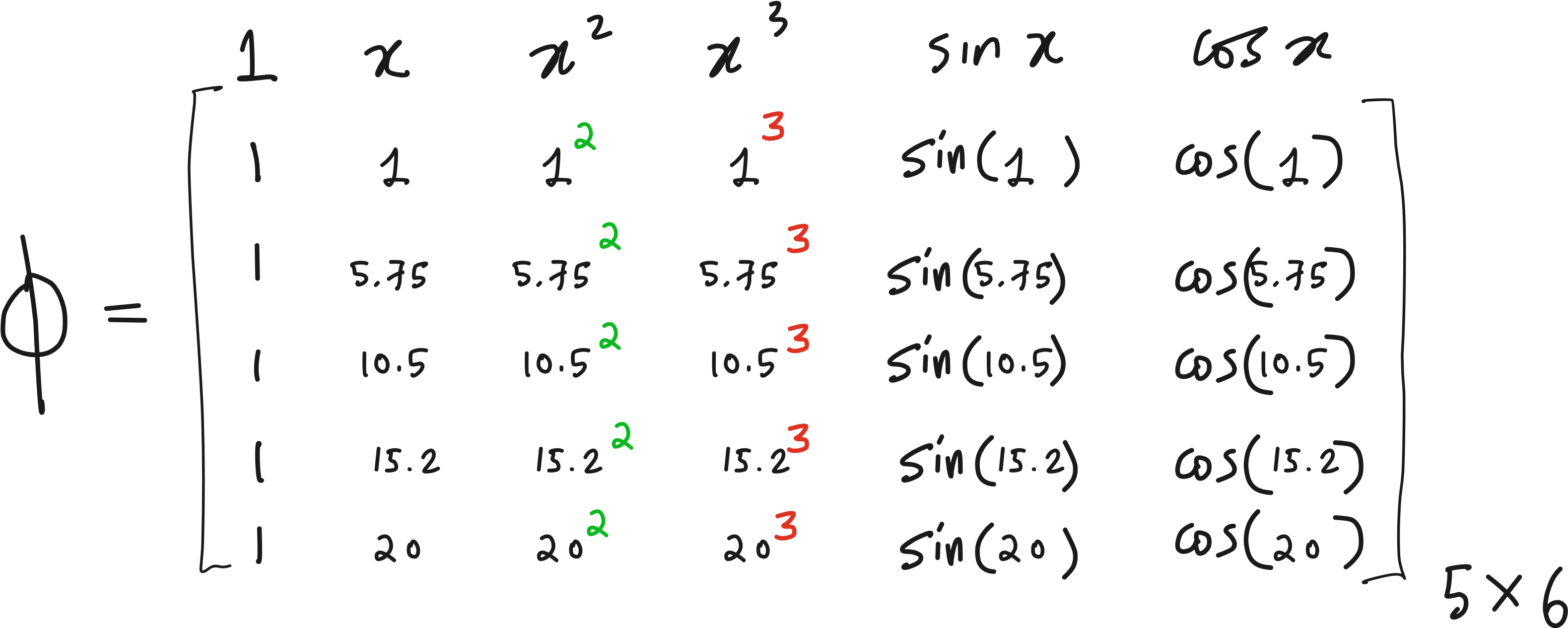
It does not assume the form. Instead, it builds a library of candidate functions:

• Constant term

• x, x^2, x^3

• sin⁡(x), cos⁡(x), log⁡(x)

It then searches for a sparse combination of these functions that can explain the data.

Sparse is the key word. Nature tends to be sparse. The real underlying equation rarely depends on all possible terms. Most are irrelevant. Symbolic regression knows this. It penalizes complexity. It favors simplicity.

The result is not just an approximation - it is an explanation.

Let us start with Data + Function Library

Step 1: Data Setup

Let’s begin with 5 data points in vector form.

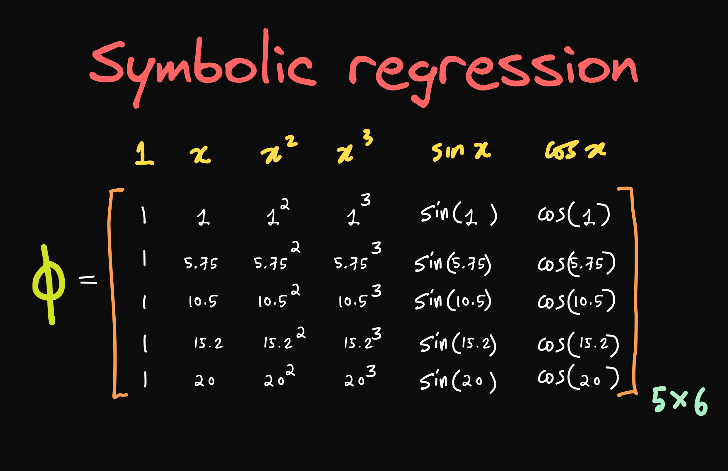
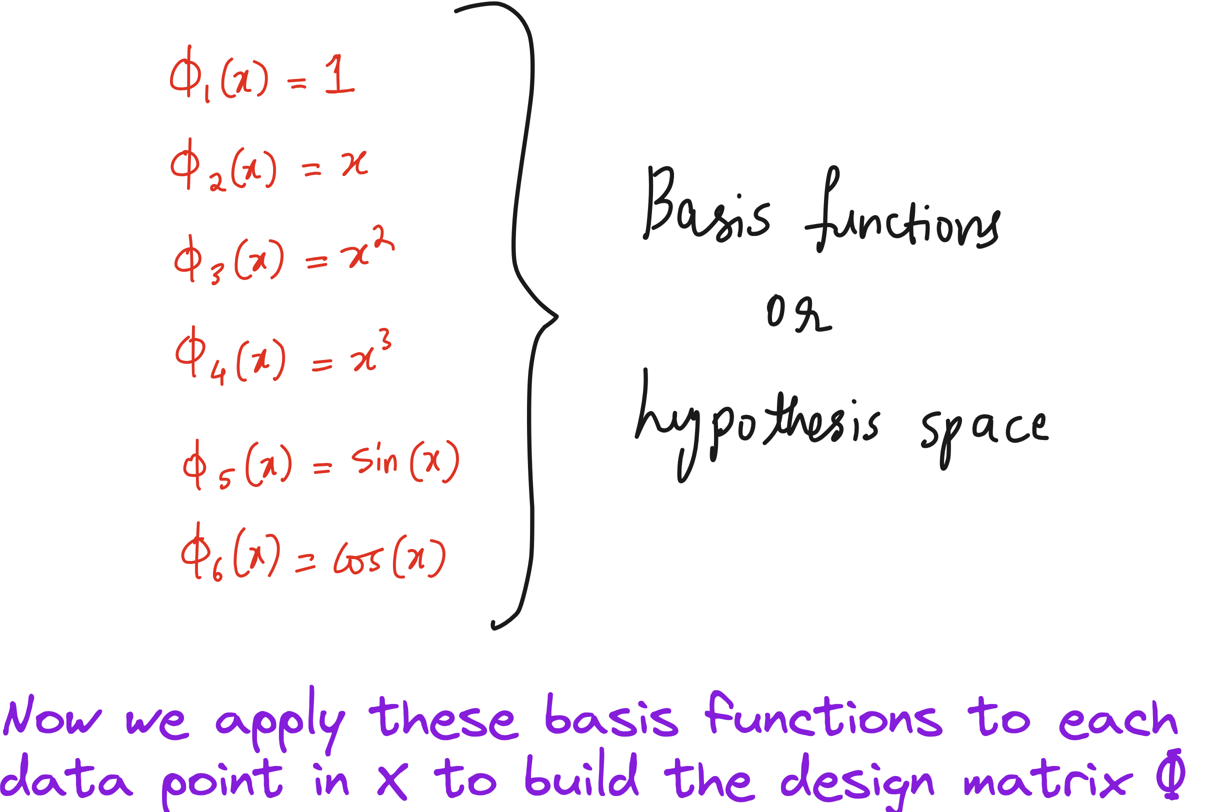
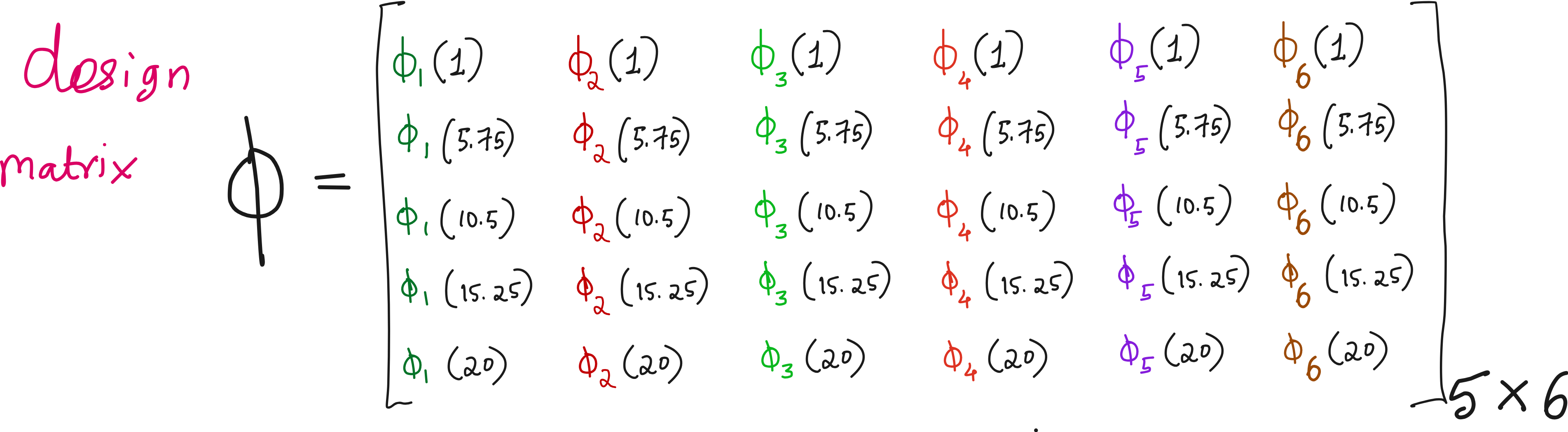
Step 2: Construct the design matrix Φ

We define a set of basis functions from our function library.

Step 3: Solve the regression problem

We want to solve the system:

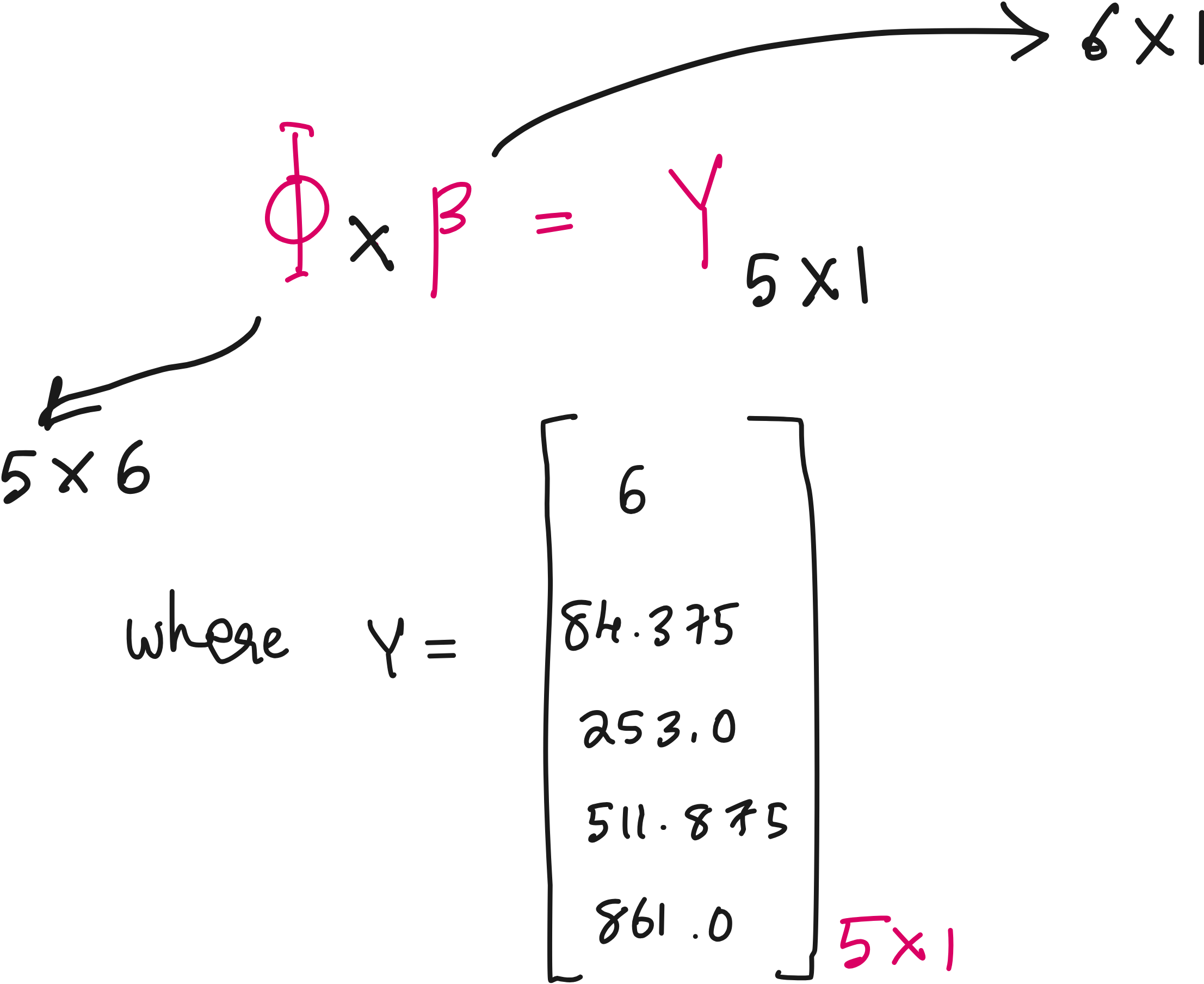
We want to solve the system:

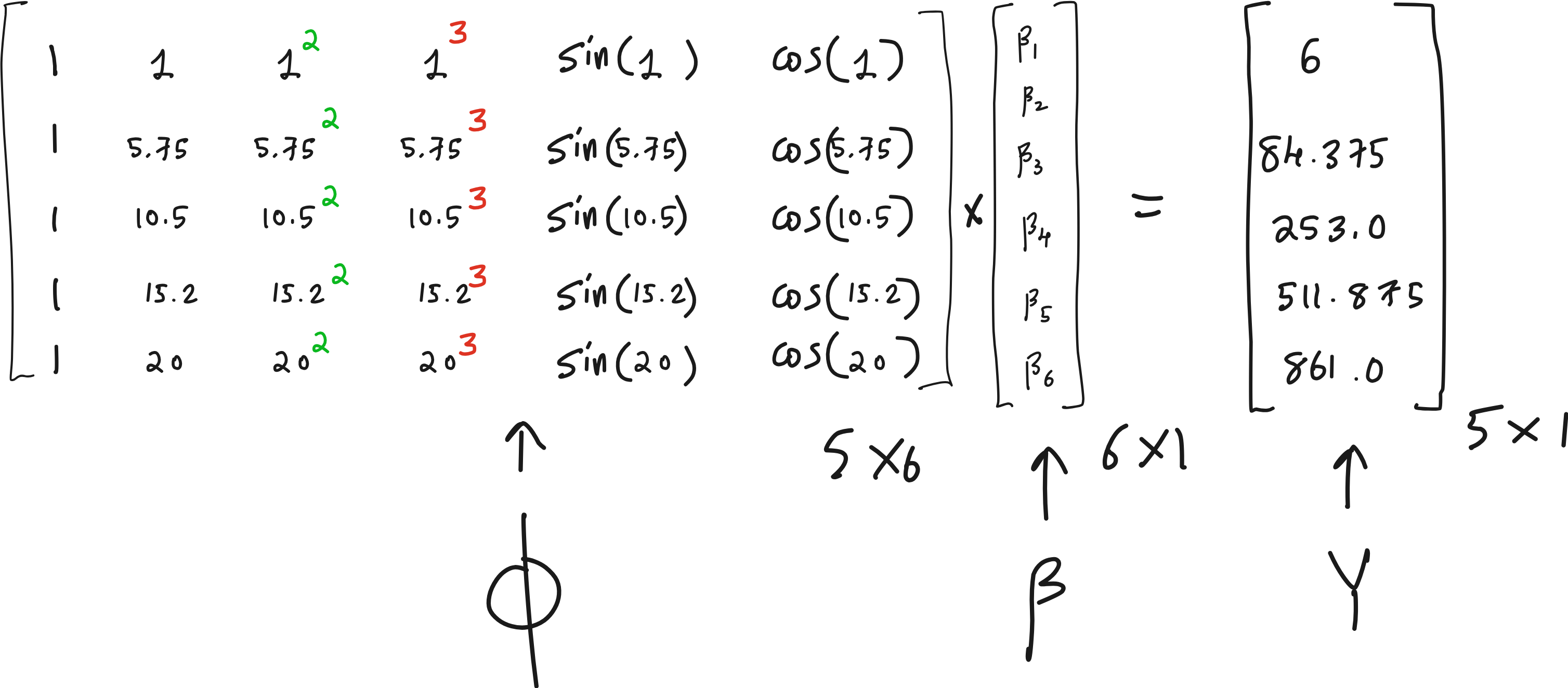
How to interpret the above equation?

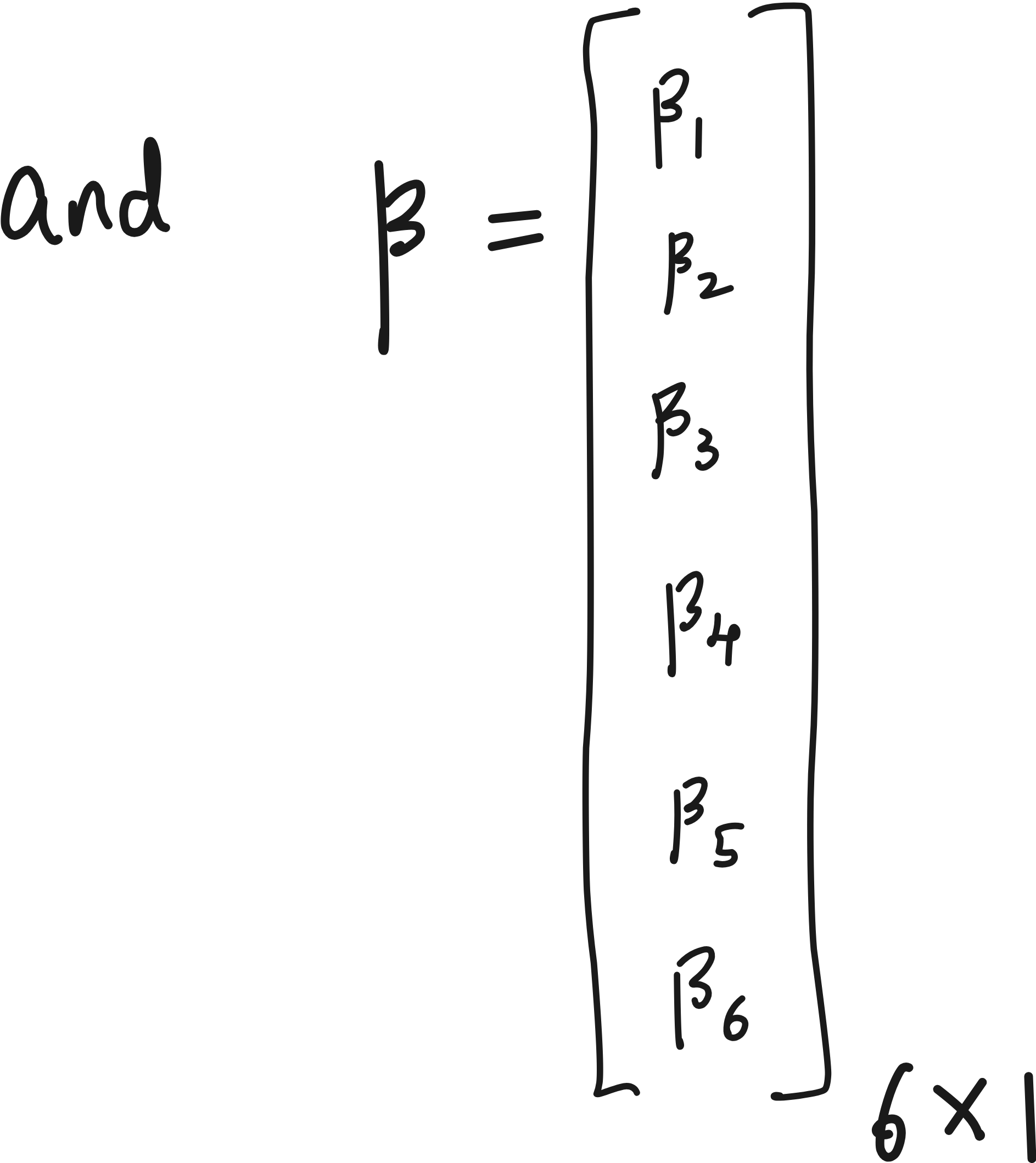
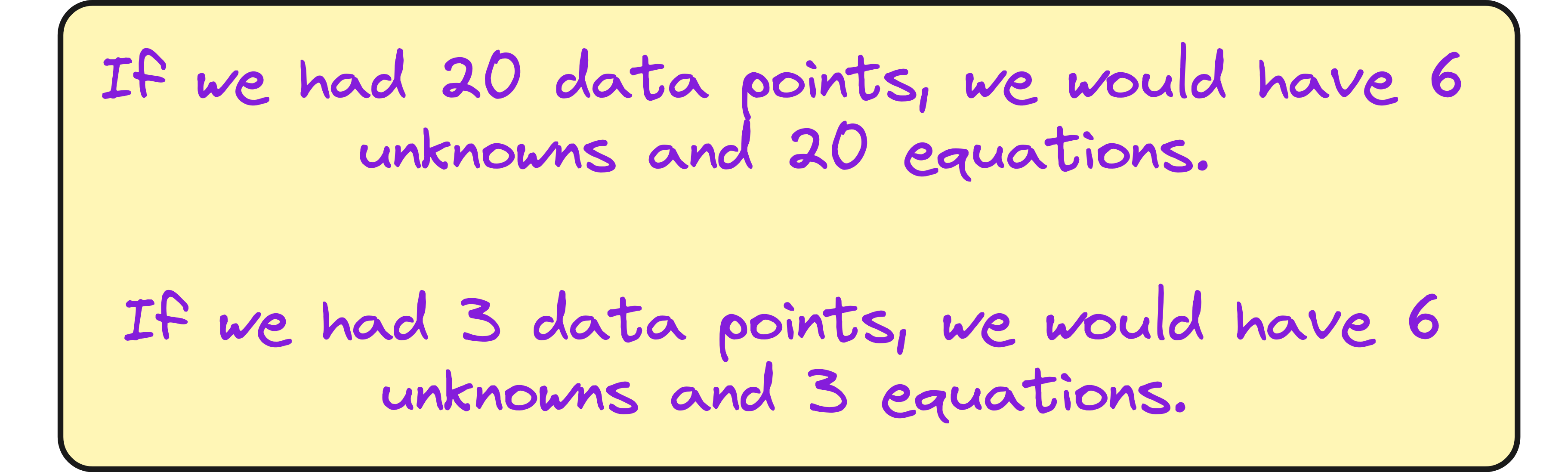
We have 6 unknowns (values of β), but 5 equations.

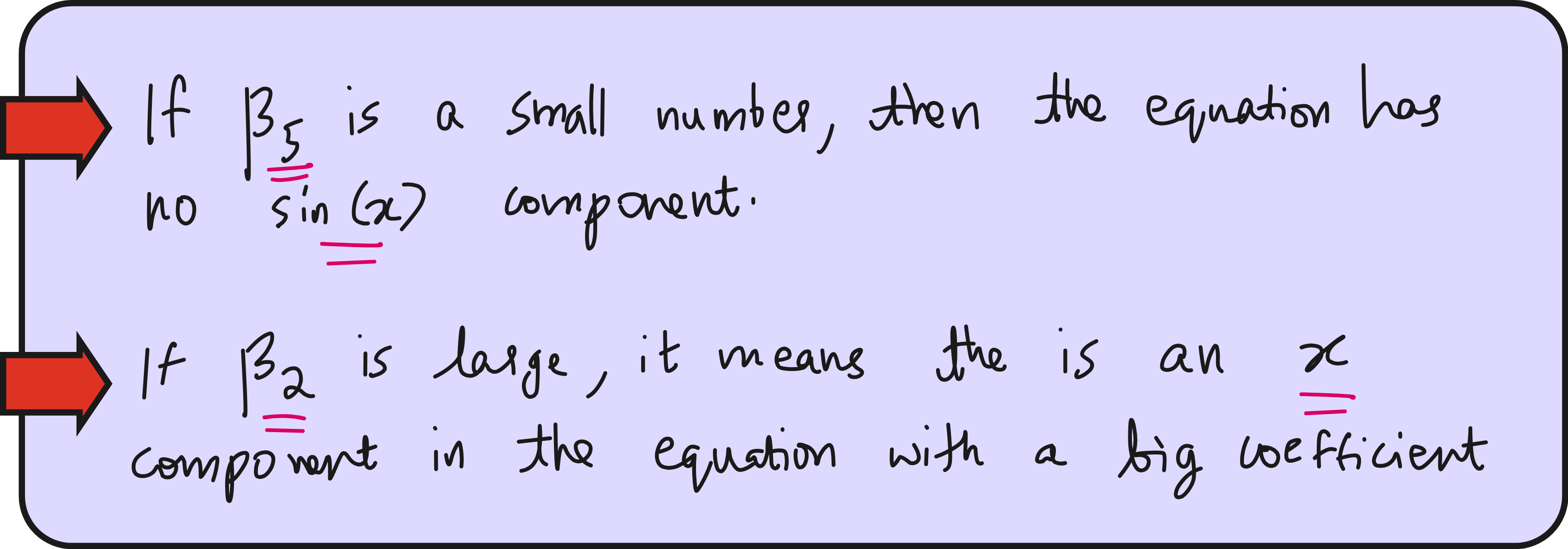
The 6 unknowns correspond to the coefficients associated with each term in our function library.

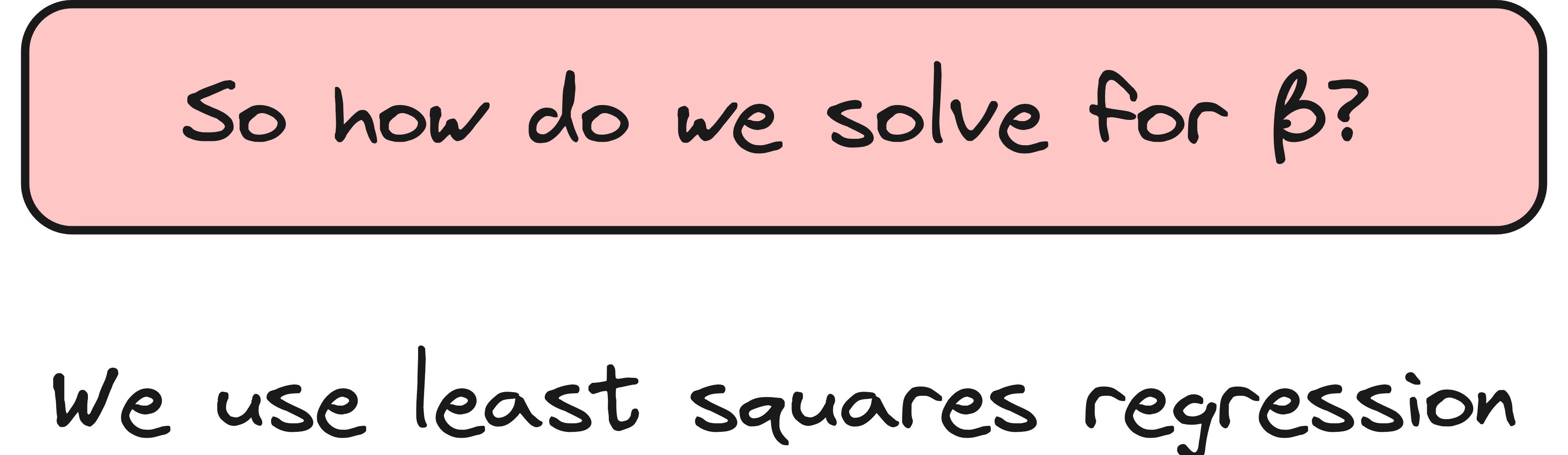
The algorithm: Least squares regression with (or without) Lasso

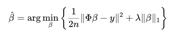
To make this work, we used a technique known as Lasso regression. It is similar to linear regression, but adds an L1​-penalty to shrink unnecessary coefficients to zero. The optimization objective is:

To simplify things, we can also do this without the penalty term.

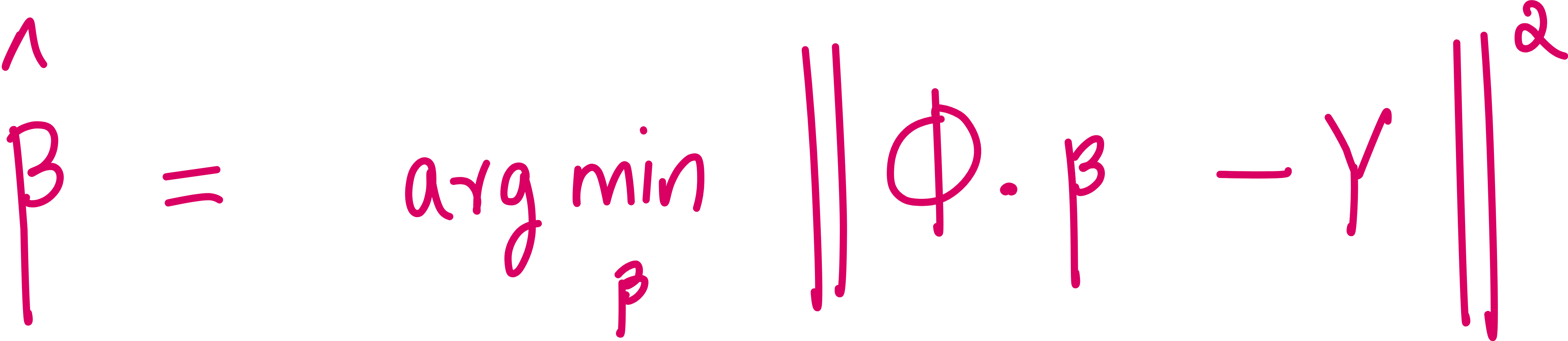
In plain English:

We are trying to find the best set of weights β so that when we combine our basis functions (in Φ) using those weights, we get as close as possible to the actual output values Y.

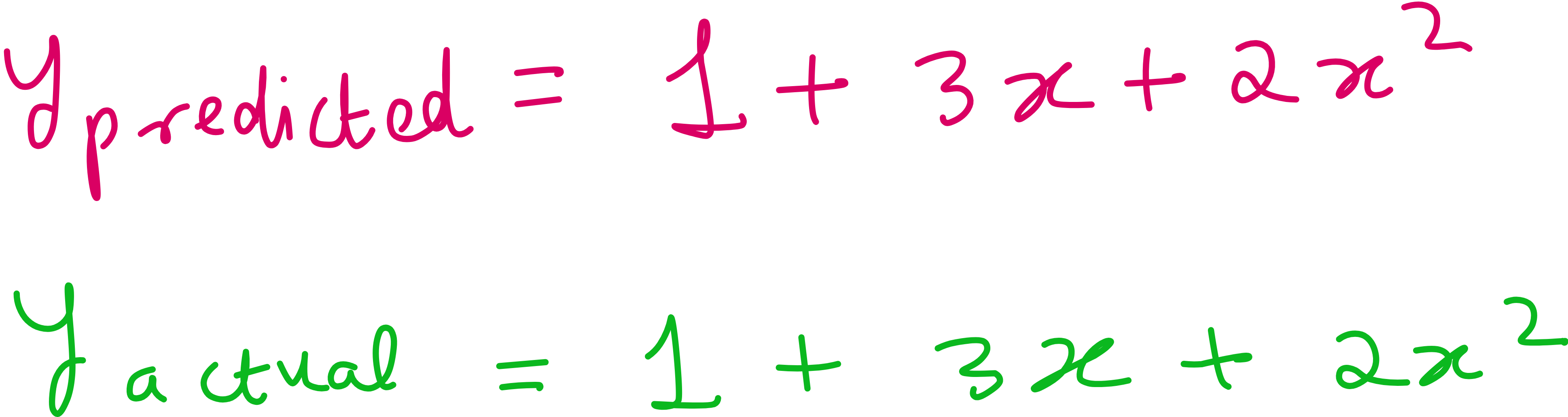
We tested this on five data points generated from the quadratic function. The function itself was unknown to the model. All it had was a list of potential terms and the raw data.

Great! Now let us implement this in code.

using LinearAlgebra  # ⬅️ Needed for dot()

# Define the data
x = range(1.0, 20.0, length=5) |> collect
y = 2 .* x.^2 .+ 3 .* x .+ 1

# Define basis functions
basis_funcs = [
    x -> 1.0,         # constant
    x -> x,           # x
    x -> x^2,         # x^2
    x -> x^3,         # x^3
    x -> sin(x),      # sin(x)
    x -> cos(x),      # cos(x)
]
basis_names = ["1", "x", "x^2", "x^3", "sin(x)", "cos(x)"]

# Construct design matrix
Φ = [f(xi) for xi in x, f in basis_funcs]  # size (n, p)

# Solve for β
β = Φ \ y

# Display results
println("Solution without Lasso penalty:")
for i in 1:p
    println("  ", round(β[i], digits=4), " * ", basis_names[i])
end

y_fitted = [sum(β[i] * basis_funcs[i](xi) for i in 1:length(basis_funcs)) for xi in x]

# Plot original data vs fitted model
plot(x, y, seriestype=:scatter, label="Original Data", xlabel="x", ylabel="y", title="Symbolic Recovery")
plot!(x, y_fitted, label="Fitted Model", linewidth=2)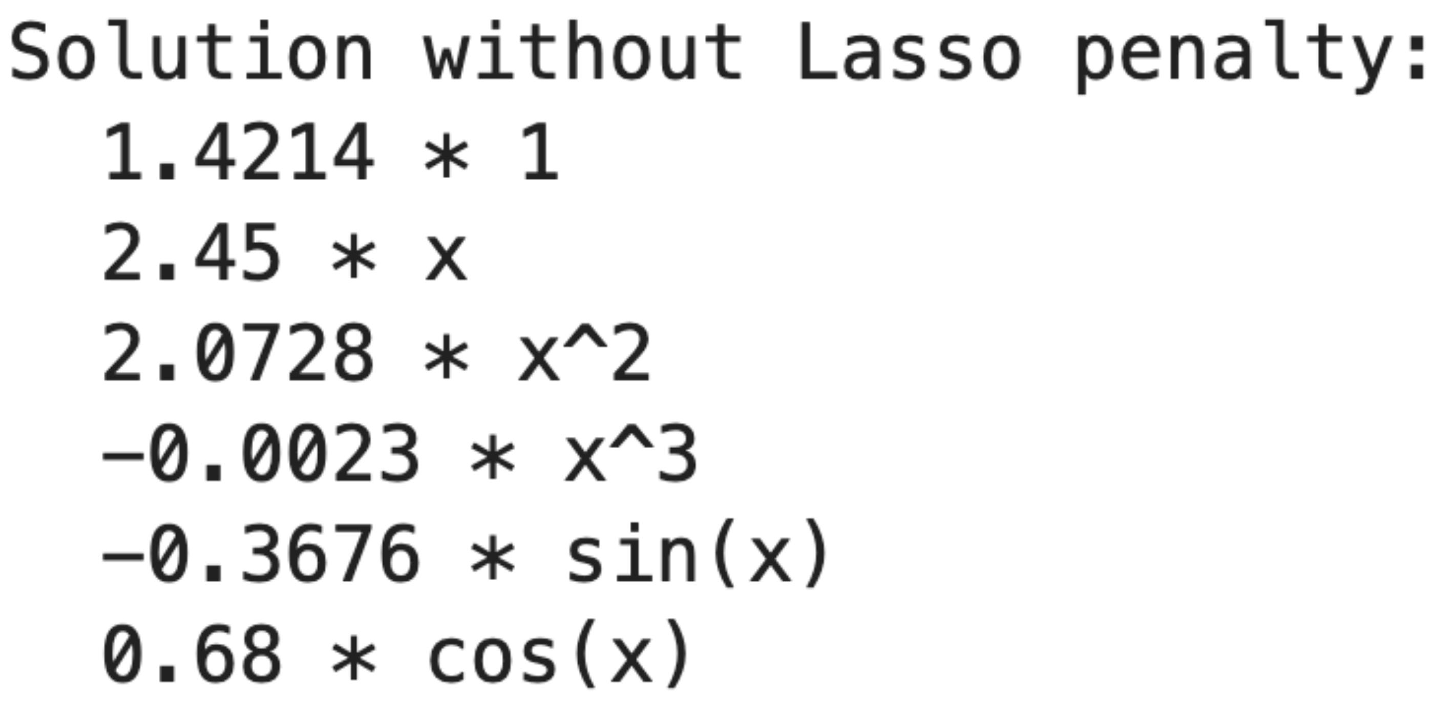

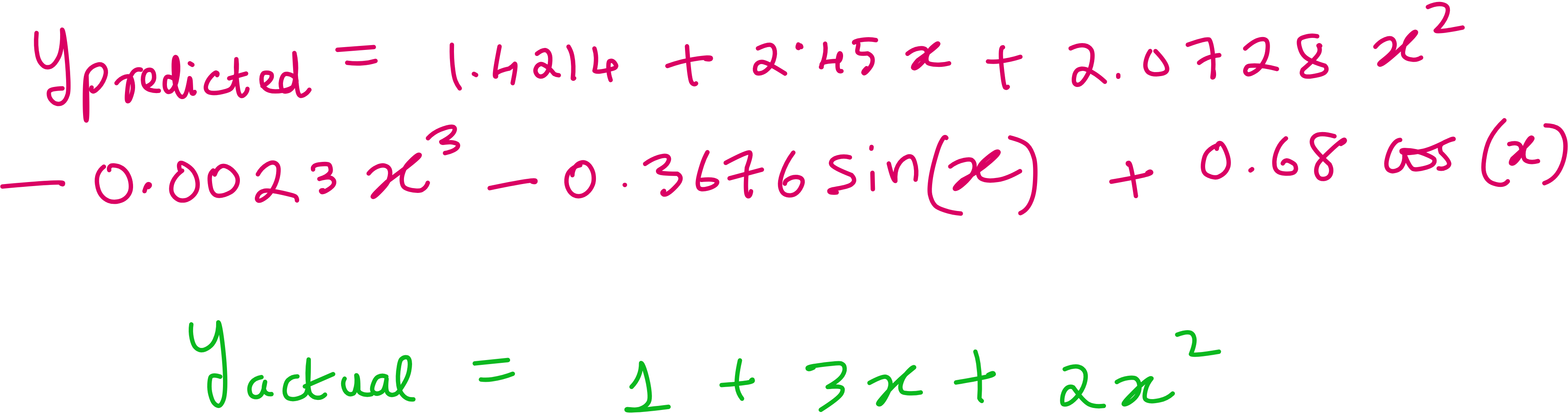
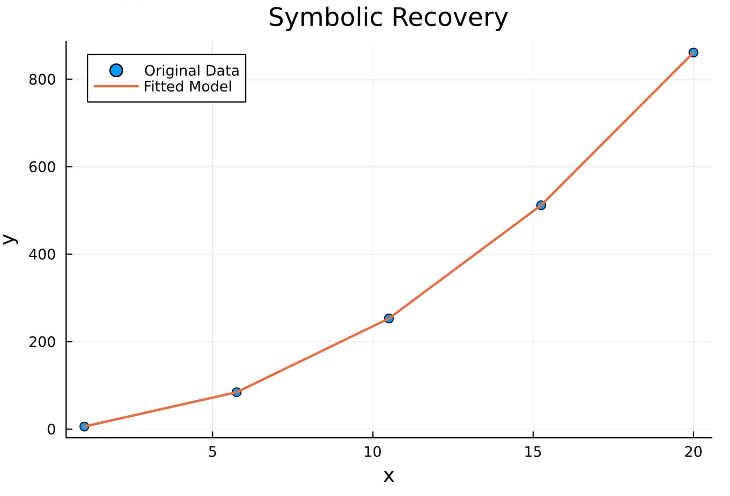
Although the fit looks great, the recovered function looks very different from the actual function. We can fix this using more input data points.

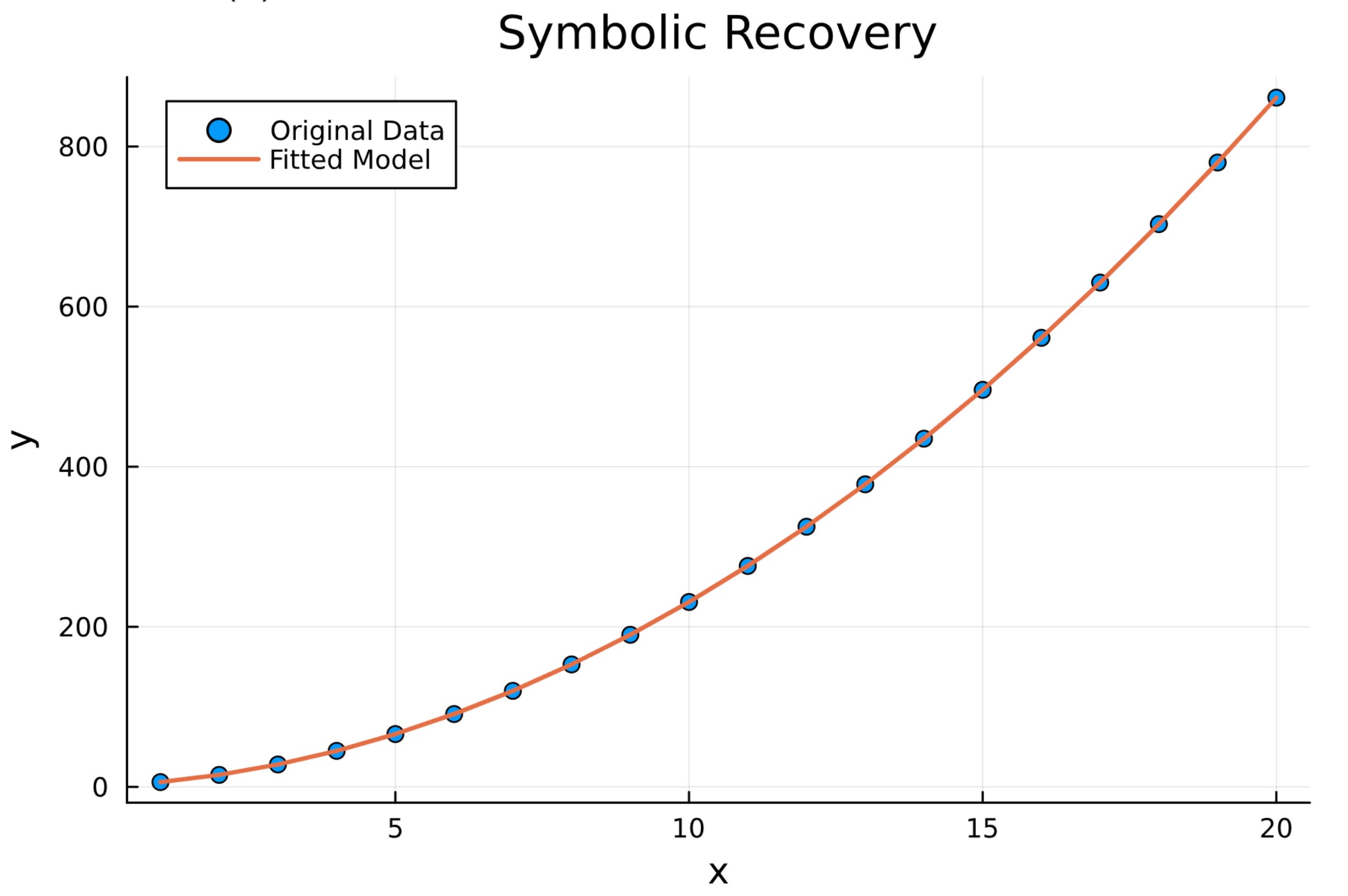
Let us consider more data points.

Modify this part of the code.

# Step 1: Define the data
x = range(1.0, 20.0, length=20) |> collect
y = 2 .* x.^2 .+ 3 .* x .+ 1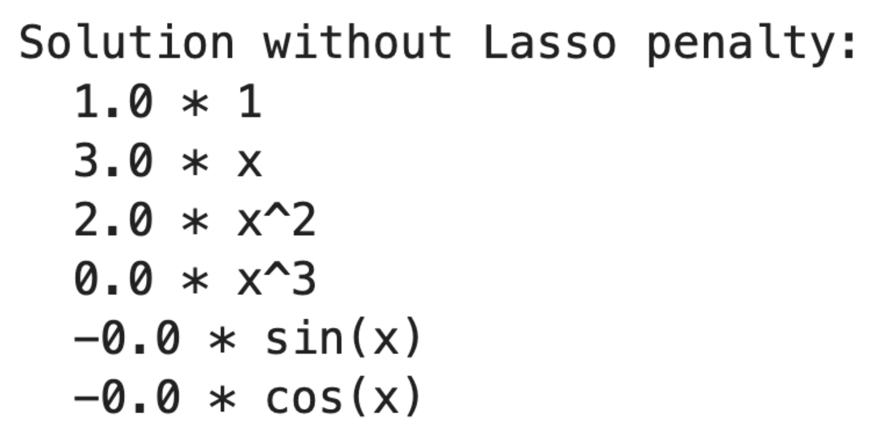

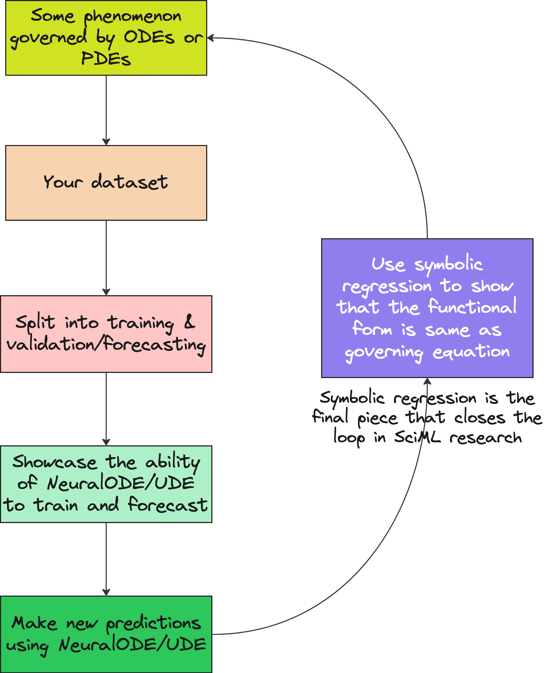
Symbolic regression is the last piece of SciML research papers.

This is NOT about quadratics

The quadratic example is just a sandbox.

What makes symbolic regression powerful is how it scales to real-world scientific discovery. Imagine having a system whose dynamics are unknown - some physical process, some biological feedback loop, some economic phenomenon. You collect data. You have no idea what is driving it.

Symbolic regression becomes your microscope.

It does not need millions of parameters. It does not hallucinate patterns. It builds equations. Sparse. Logical. Readable.

That is the edge. Interpretability at its core.

You do not get a model. You get an equation.

Why this matters

In a world obsessed with deep learning, interpretability often gets sacrificed on the altar of performance. Neural networks give you answers, but not understanding. They predict, but they do not explain.

Symbolic regression does the opposite.

It is not about error rates.

It is about clarity.

It is about machines that do not just learn - they reason. They extract structure. They write math.

And that makes them not just accurate, but trustworthy.

A new kind of scientific tool

As machine learning moves deeper into scientific domains - physics, chemistry, biology - the ability to discover structure will matter more than ever.

Symbolic regression is not a toy.

It is a telescope aimed at the laws of the universe.

It allows us to reverse-engineer what we once assumed had to be known in advance. From data to model. From chaos to clarity.

In the end, the power of symbolic regression is not in solving for coefficients.

It is in reminding us that data hides stories -

and that some stories are still written in equations.

YouTube lecture

Interested in learning AI/ML live from us?

Check this out: https://vizuara.ai/live-ai-courses

Here is a simple diagram that summarizes it all: