
Variational Autoencoders explained from scratch
VAEs explained from first principles

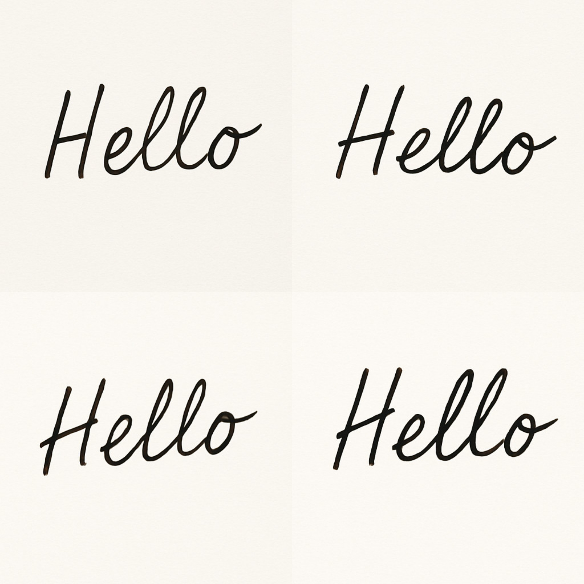
Let us start with a simple example. Imagine that you have collected handwriting samples from all the students in your class (100). Let us say that they have written the word “Hello.”
Now, students will write the word “hello” in many different ways. Some of them will write words which are more slanted towards the left. Some of them will write words which are slanted towards the right.
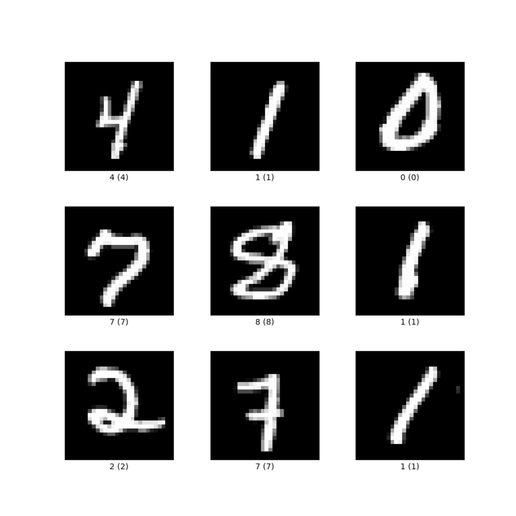
Some words will be neat, some words will be messy. Here are some of the samples of the words “hello”.
Now, let us say that someone comes to you and asks,
“Generate a machine which can produce samples of handwriting for the word ‘hello’ written by students of your class.”
HOW WILL YOU SOLVE THIS PROBLEM?
Part 1
The first thing that will come to your mind is: What are the hidden factors that determine the handwriting style?
Each student’s handwriting depends on many hidden characteristics:
How much pressure they apply?
Whether they write slanted
Whether their letters are wide or narrow
How fast they write?
How neat they are?
These are not directly seen in the final image, but they definitely cause the shape of the letters.
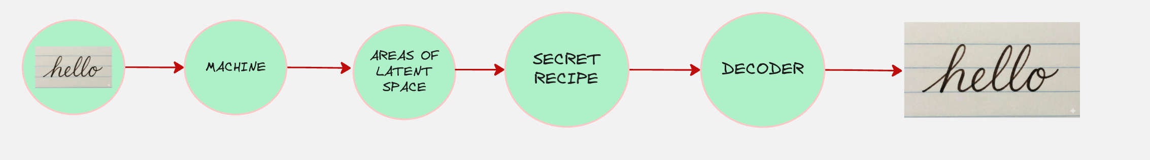
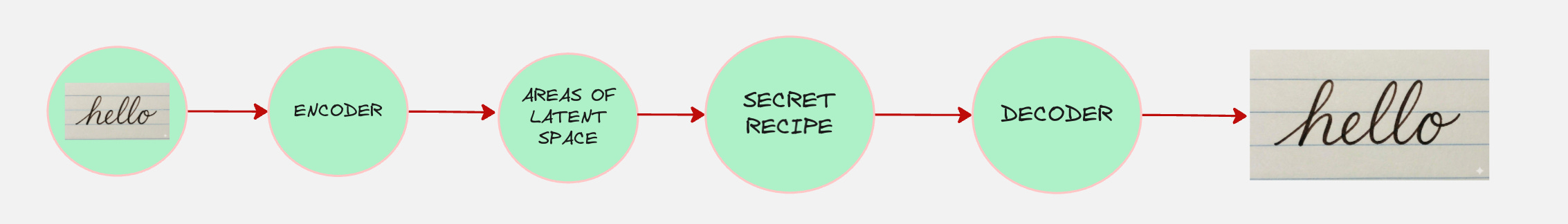
In other words, every handwriting has a secret recipe that determines the final shape of the handwriting.
For example, this person writes slightly tilted, thin strokes, medium speed, moderate neatness.
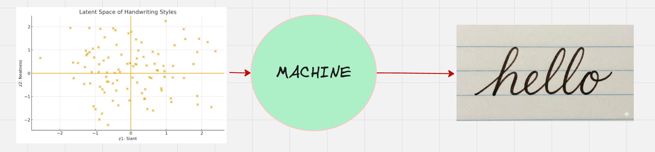
So, the general architecture of the machine looks as follows:
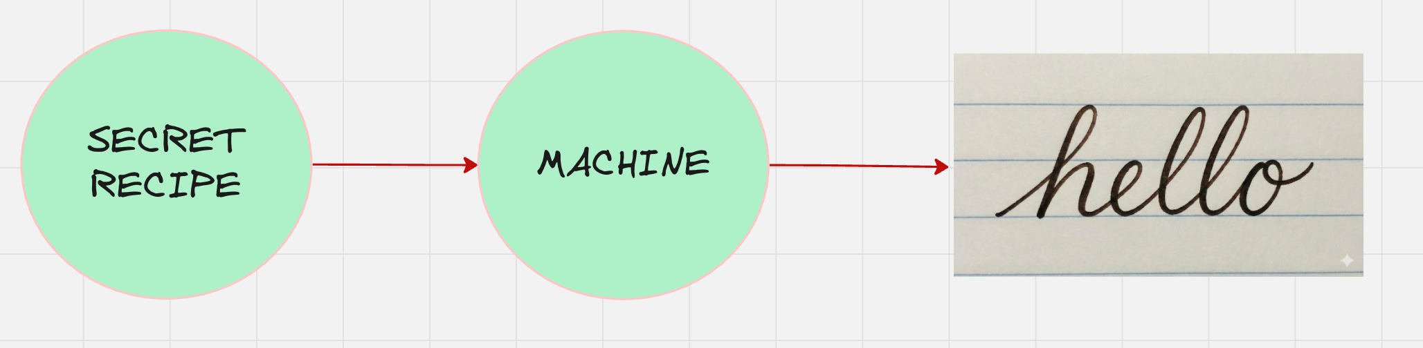
This secret recipe is something which is called as the latent variable. Latent variables are the hidden factors that determine the handwriting style.
These variables are denoted by the symbol “z”.
The latent variables (z) captures the essence of how the handwriting was formed.
Let us try to understand the latent variables for the handwriting example.
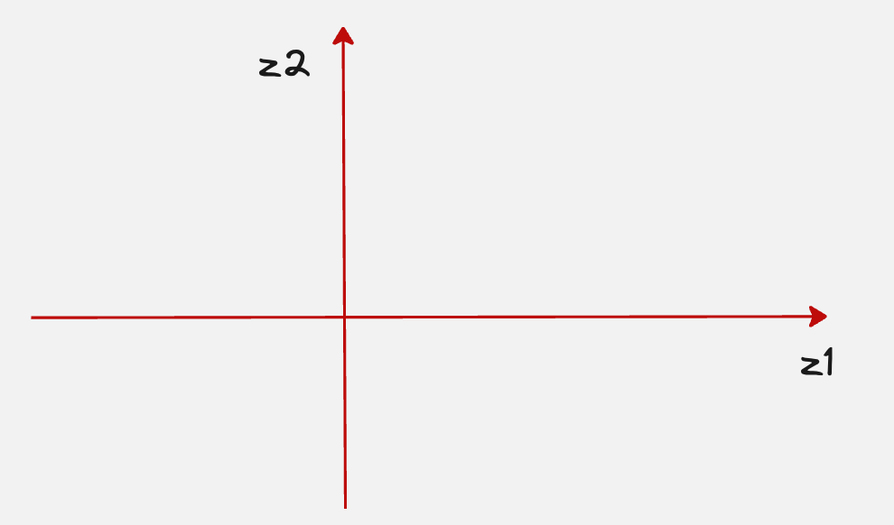
Let us assume that we have two latent variables:
One which captures the slantness
One which captures the neatness of the handwriting
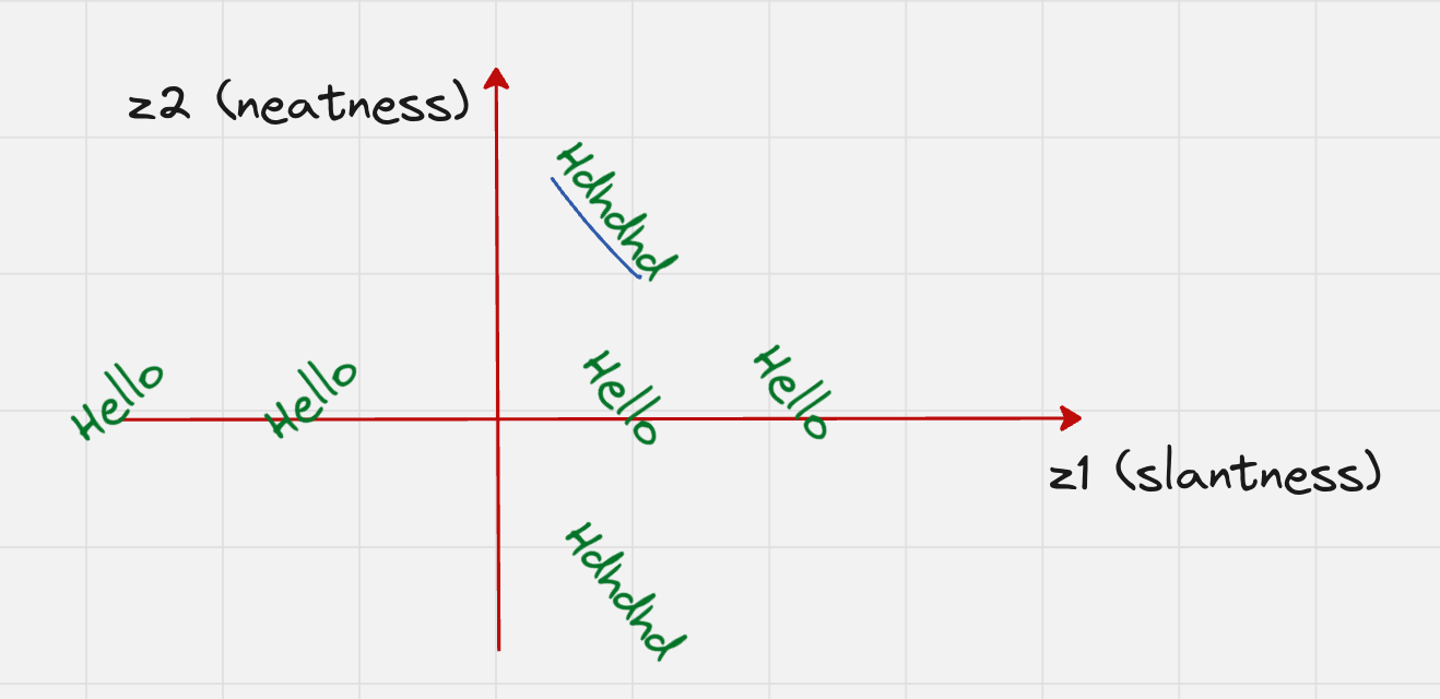
From the above graph, you can see that both axes carry some meaning.
Words which are on the right-hand side are more slanted towards the right
Words which are on the left-hand side are more slanted towards the left
Also, words which are on the top or down are very messy.
So, we can see that every single point on this plane corresponds to a specific style of handwriting.
In reality, the distribution for all 100 students in your class might look as follows.
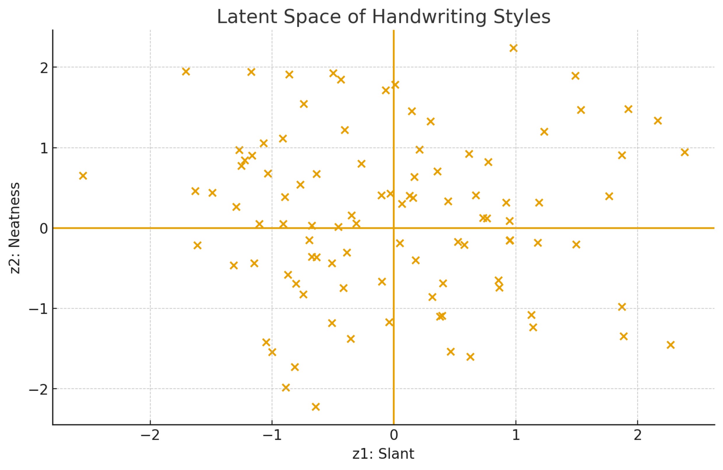
We observe that each handwriting image is compressed into just two numbers: slant and neatness.
Similar handwritings end up as nearby points in this 2D latent space.
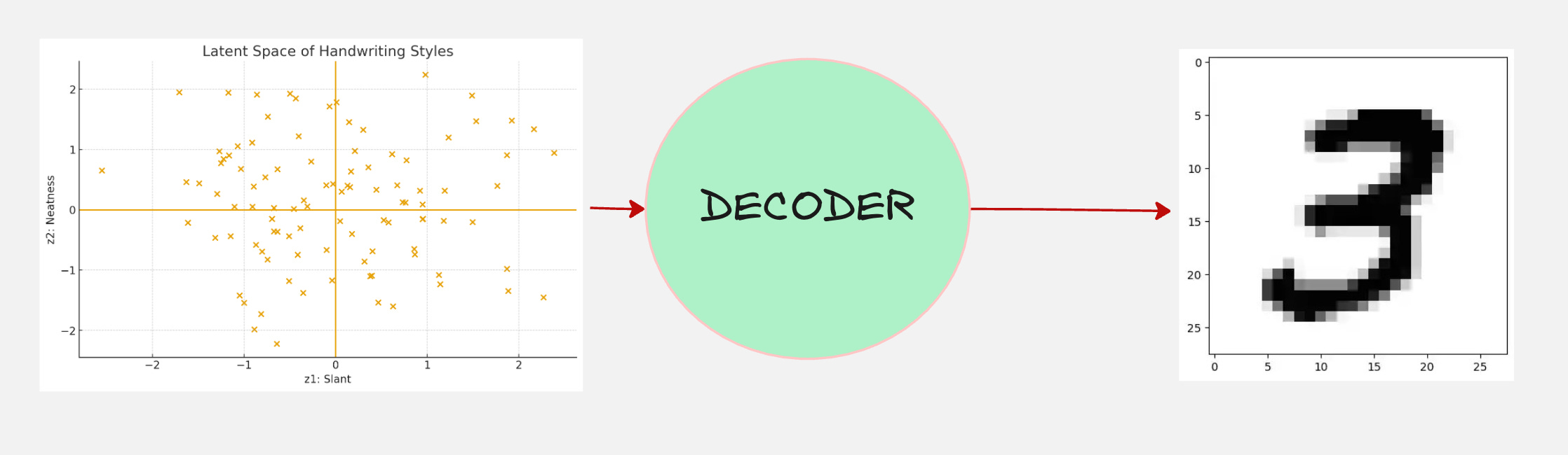
Now, let us feed this to our machine which generates the handwriting.
There is another word for this machine, which is called the “decoder”
Let us see a visual animation to see how the decoder works for the above example:
So far, we have just used the word “decoder” to generate samples from the latent variables, but what is this decoder exactly and how are the samples generated?
Let us say, instead of generating handwriting samples our task is to generate handwritten digits.
Again, we start with the same thinking process. What are the hidden factors that determine the shape of the handwritten digits?
And we create a latent space with the latent variables.
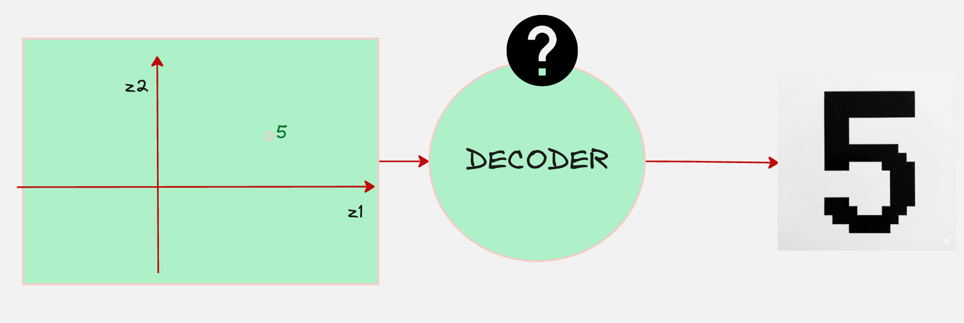
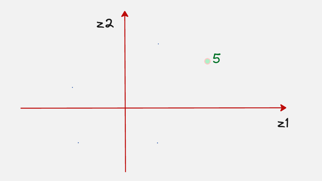
Just as before, let us assume that there are two latent variables.
Now let’s assume that we have chosen a point in the latent space which corresponds to the number 5.

The main question is, how do we generate the actual sample for the digit 5 once we pass this to the decoder?
First, let us begin by dividing the image of the digit 5 into a bunch of pixels like follows.

Each pixel corresponds to a number. For example, white pixels correspond to 1 and black pixels correspond to 0.
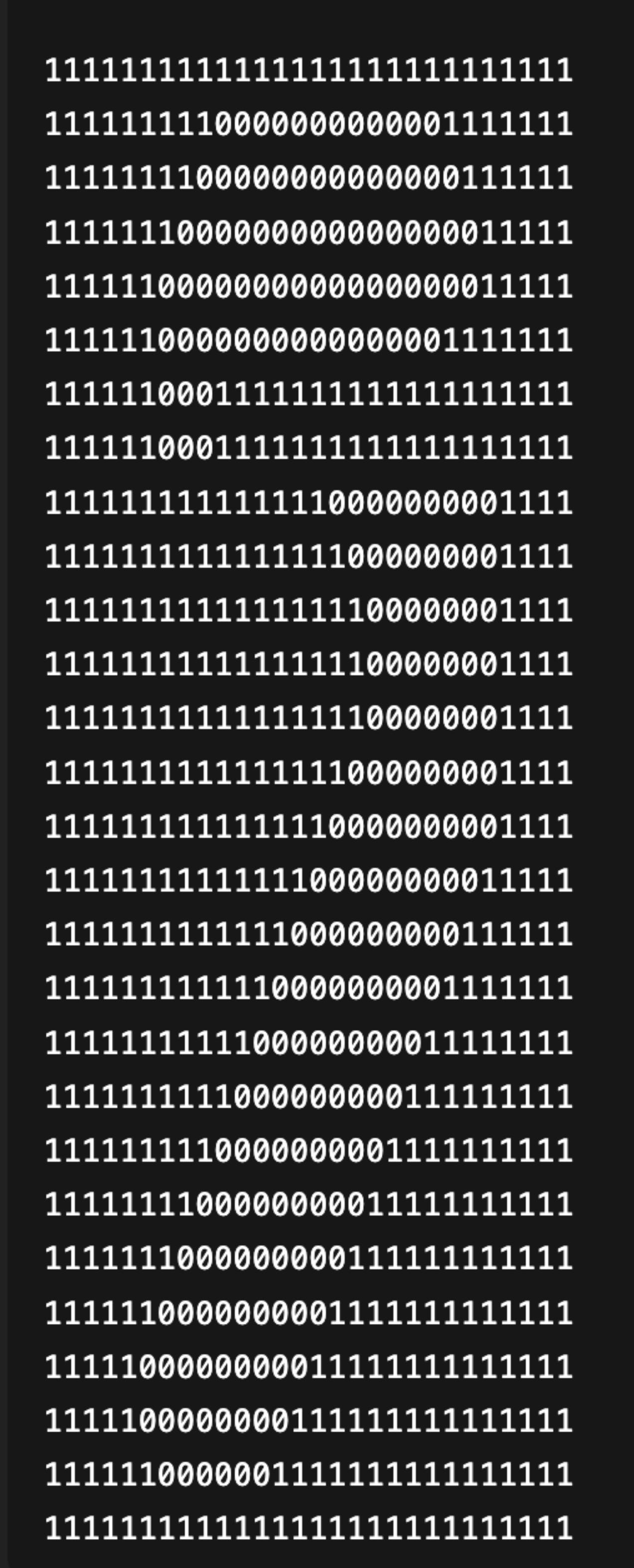
So it looks like all we have to do is output a number, either 0 or 1, at the appropriate location so that we get the shape 5.
However, there is one drawback of this approach: with this approach, we will get a fixed shape 5 every time. We will not get variations of it.
But we do want to get variations of number 5. Remember in all the image generation applications, in the same prompt, we can get different variations of the image? We want exactly that.
So instead of outputting a single number, what if you could output a probability density?
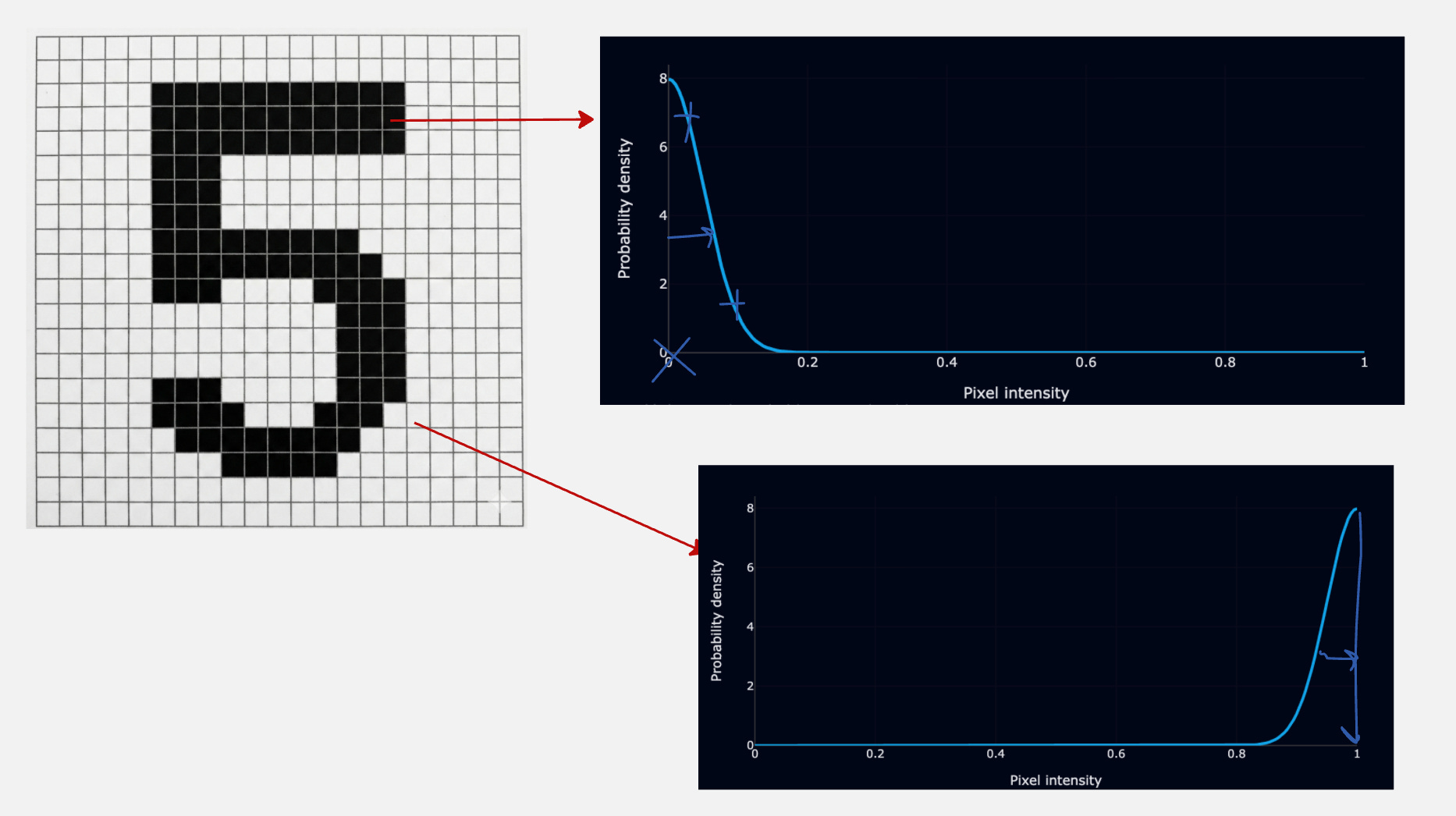
So, the actual value of the pixel intensity becomes the mean, and we add a small standard deviation to it.
Let us look at a simple visualization to understand this better.
Part 2:
Okay, we have covered one part of the story which explains the decoder.
Now let’s cover the second part so that we get a complete picture.
If you paid close attention to the first part, you will understand that we have made a major assumption.
Remember when we talked about the handwritten digit 5, we said that let us assume that this part of the latent space corresponds to the digit 5.
But how do we know this information beforehand?
How do we know which part of the latent space to access to generate the digit 5?
One option is to access all possible points in the latent space, generate an image for it using our decoder distribution, and see which images match closely to the digit 5.
But this does not make sense. This is completely intractable and not a practical solution.
Wouldn’t it be better if we knew which part of the latent space to access for the type of image we want to generate?
Let us see if we build another machine to do that.
If we do this, we can connect both these machines together.
This “machine” is also called as the encoder
Have a look at the video below, which explains visually why the encoder is necessary. It also explains where the word “Variational” in “Variational Autoencoders” comes from.
These two stories put together form the “Variational Autoencoder”
Before we understand how to train the variation auto-encoder, let us understand some mathematics:
Formal Representation for VAEs
In VAEs we distinguish between two types of variables:
Observed variables (x), which correspond to the data we see, and latent variables (z) (which capture the hidden factors of variation).
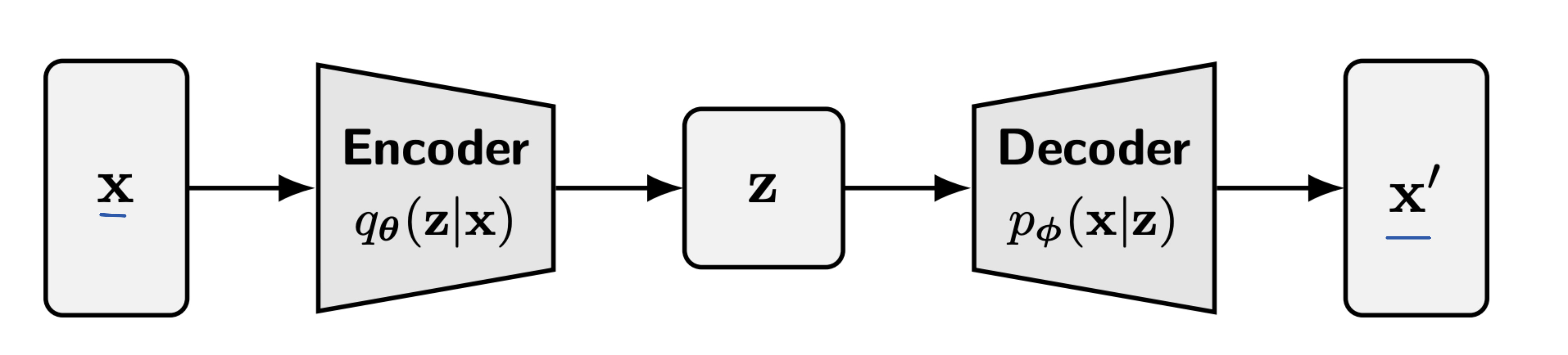
The decoder distribution is denoted as follows:
The notation reads: Probability of x given z.
The encoder distribution is denoted as follows:
The notation reads: Probability of z given x.
The schematic representation for the variational autoencoder can be drawn as follows:
Training of VAEs
From the above diagram, we immediately see that there are two neural networks: the encoder and decoder, which we have to train.
The critical question is, what is the objective function that we want to optimize in this scenario?
Let us think from first principles. We started off with the objective that we want our probability distribution to match the true probability distribution of the underlying data.
This means that we want to maximize the following:
This makes sense because, if the probability of drawing the real samples from our predicted distribution is high, we have done a good job in modeling the true distribution.
But how do we calculate the above probability?
Okay, let us start by using the following formula:
We have looked at the same analogy in the visual animation which we saw before.
It essentially means that we look at all possible variations in the hidden factors and sum over all the probabilities over all these hidden factors.
However, this is mathematically intractable.
How can we possibly go over every single point in the latent space and find out the probability of the sample drawn from that point being real?
This does not even make use of the encoder.
So now we need a computable training objective.
Training via the Evidence Lower Bound
Have a look at the video below:
The idea is to find a term which is always less than the true objective, so if we maximize this term, our true objective also will be maximized.
The evidence lower bound is made up of two terms given below.
Term 1: The Reconstruction Term
This term essentially says that the reconstructed output should be similar to the original input. It’s quite intuitive.
Term 2: The Regularization Term
This term encourages the encoder distribution to stay as close as possible to the assumed distribution of the latent variables, which is quite commonly a Gaussian distribution.
The reason why the latent space is assumed to be Gaussian in my opinion is that we assume that all real-world processes have variables which have a typical value and they have extremes where the probability is generally less.
Practical example
Let us take a real-life example to understand how the ELBO is used to train a Variational AutoEncoder.
Our task is to train a variation autoencoder to predict the true distribution that generates MNIST handwritten digits and generate samples from that distribution.
First, let us start by understanding how we will set up our decoder. Remember our decoder setup looks as follows:
The decoder is a distribution which maps from the latent space to the input image space.
For every single pixel, the decoder should give as an output the mean and the variance of the probability distribution for that pixel.
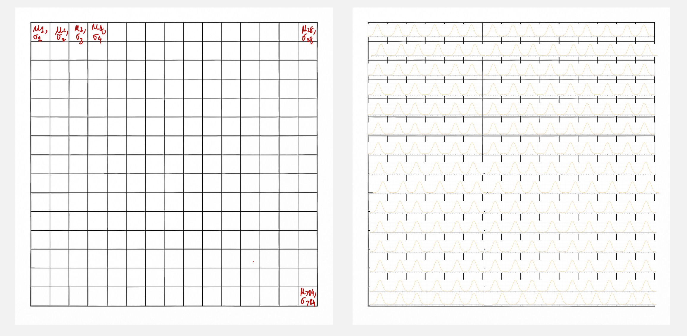
Hence, the decoder neural network should do the following:
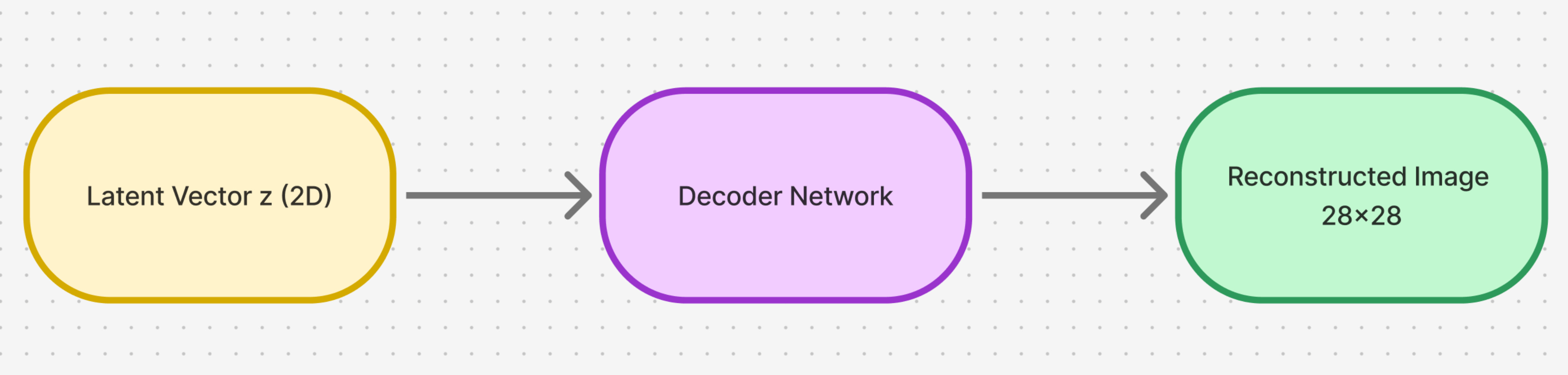
We use the following decoder network architecture:
Okay, now we have the decoder architecture in place, but remember we need the second part of the story, which is the encoder as well.
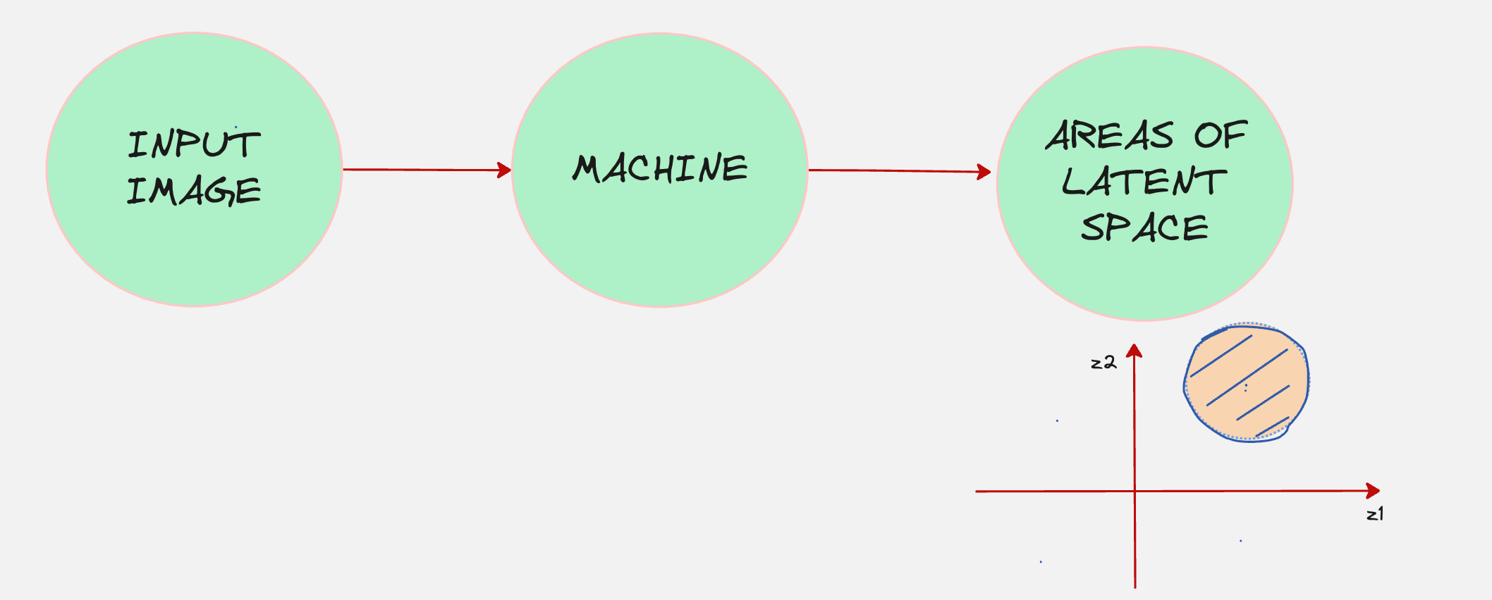
Our encoder process looks something as follows:
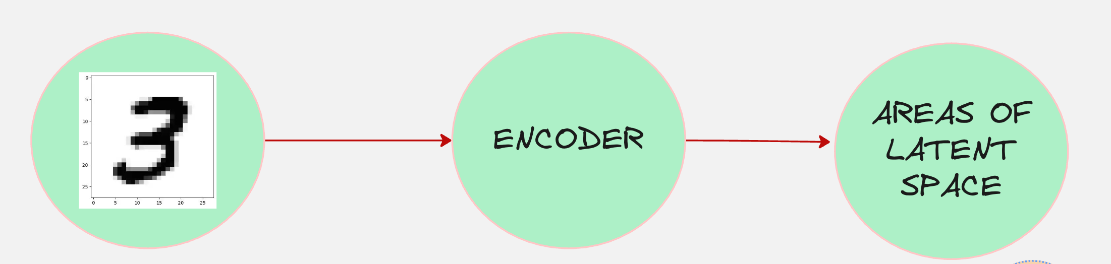
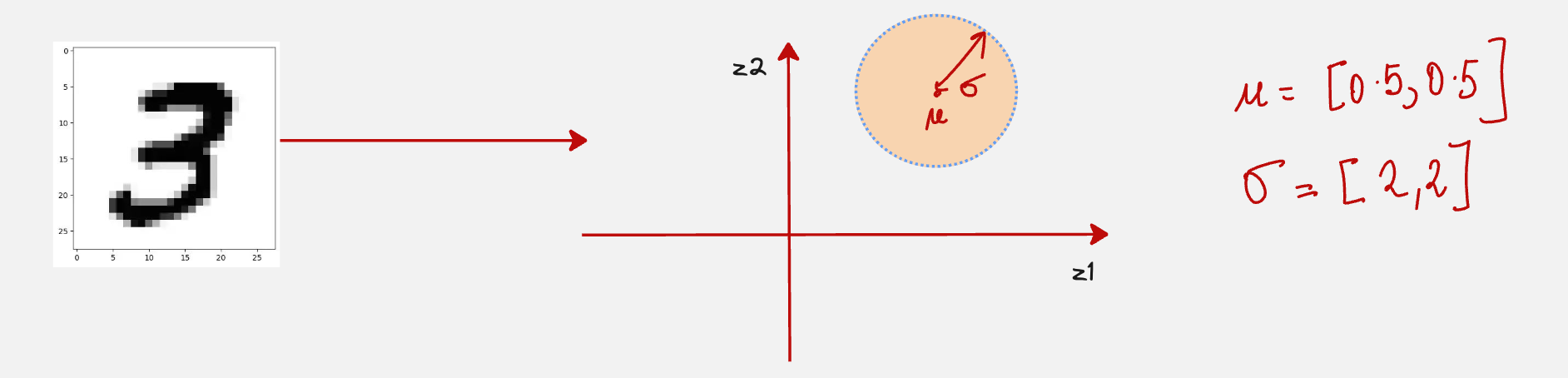
The encoder tells us which areas of the latent space the input maps to. However, the output is not given as a single point;
It is given as a distribution in the latent space.
For example, the image 3 might map onto the following region in the latent space.
Hence, the encoder neural network should do the following:
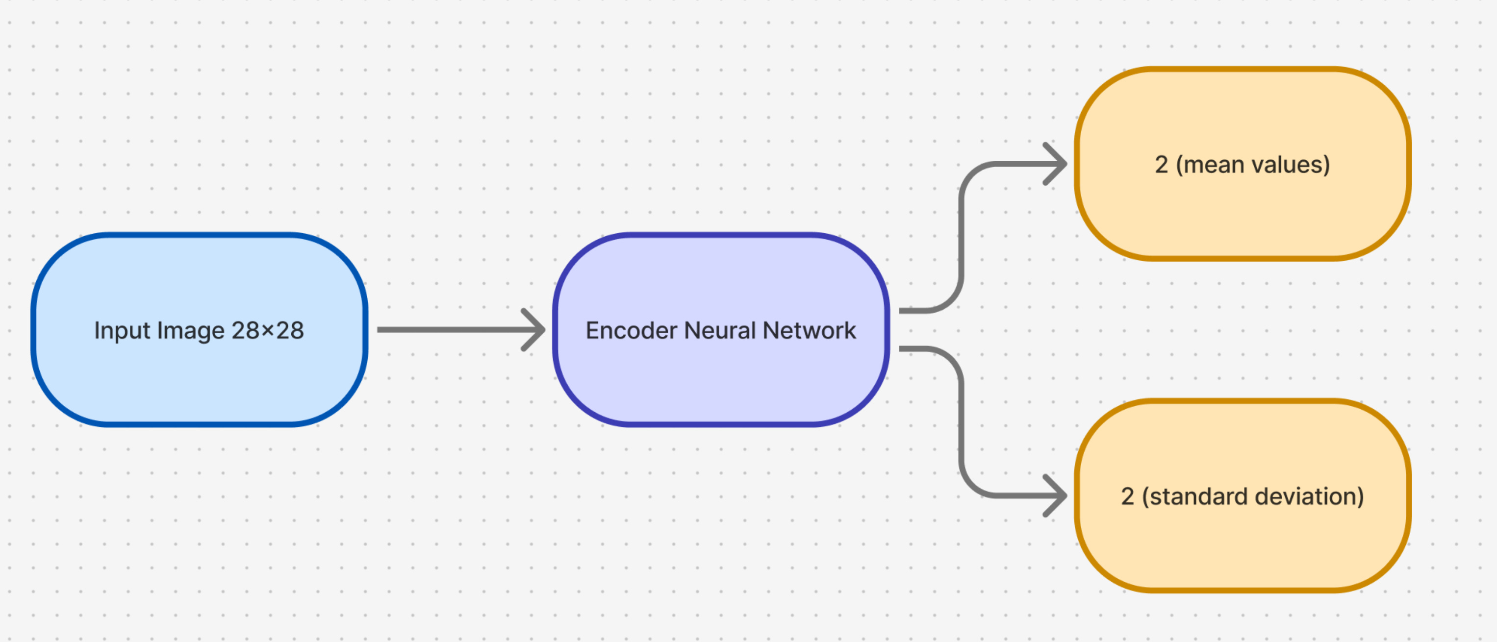
We use the following encoder architecture:
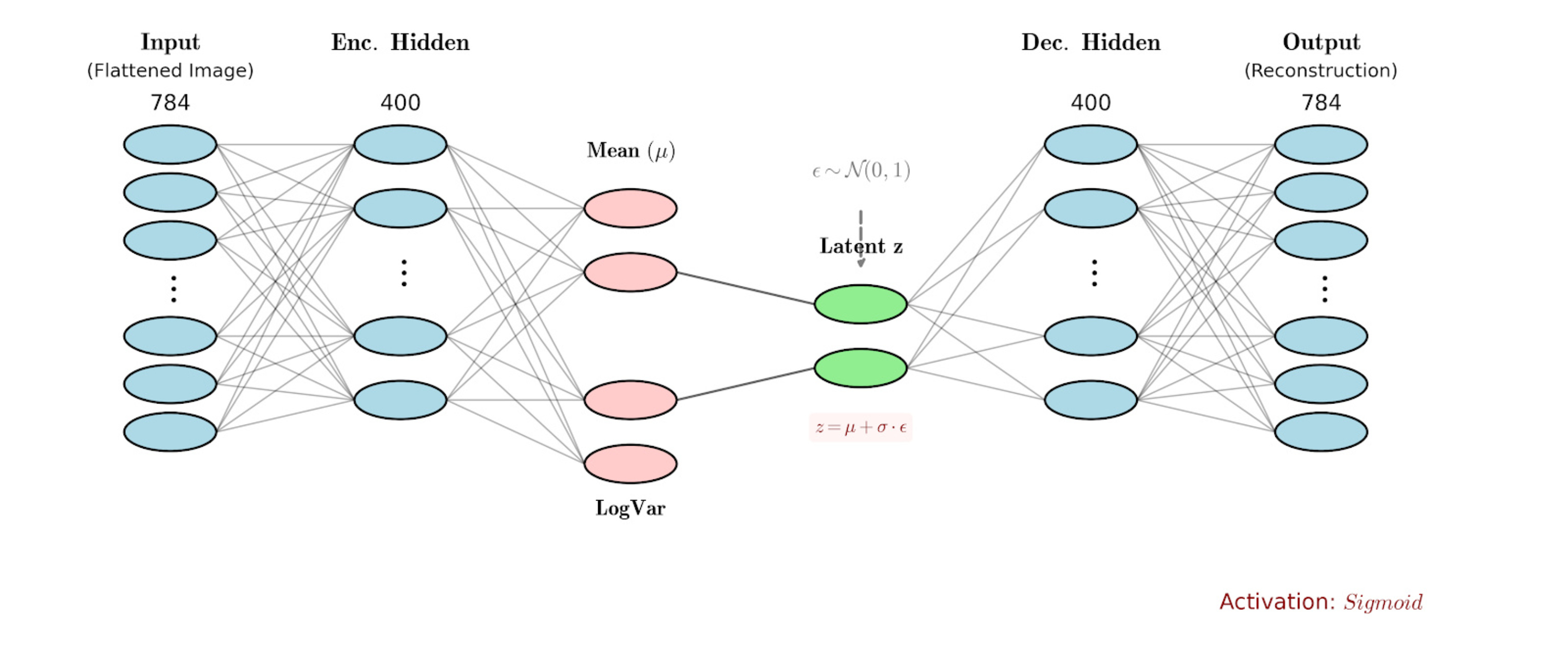
The overall encoder-decoder architecture looks as follows:
Now, let us understand how the ELBO loss is defined.
Remember the ELBO loss is made up of two terms:
The Reconstruction term
The Regularization term
First, let us understand the reconstruction loss.
The goal of the reconstruction loss is to make the output image look exactly the same as the input image.
This compares every pixel of the input with the output. If the original pixel is black and the VAE predicts white, the penalty is huge. If the VAE predicts correctly, the penalty is low.
Hence, the reconstruction loss is simply written as the binary cross-entropy loss between the true image and the predicted image.
Now, let us understand the KL-Divergence Loss:
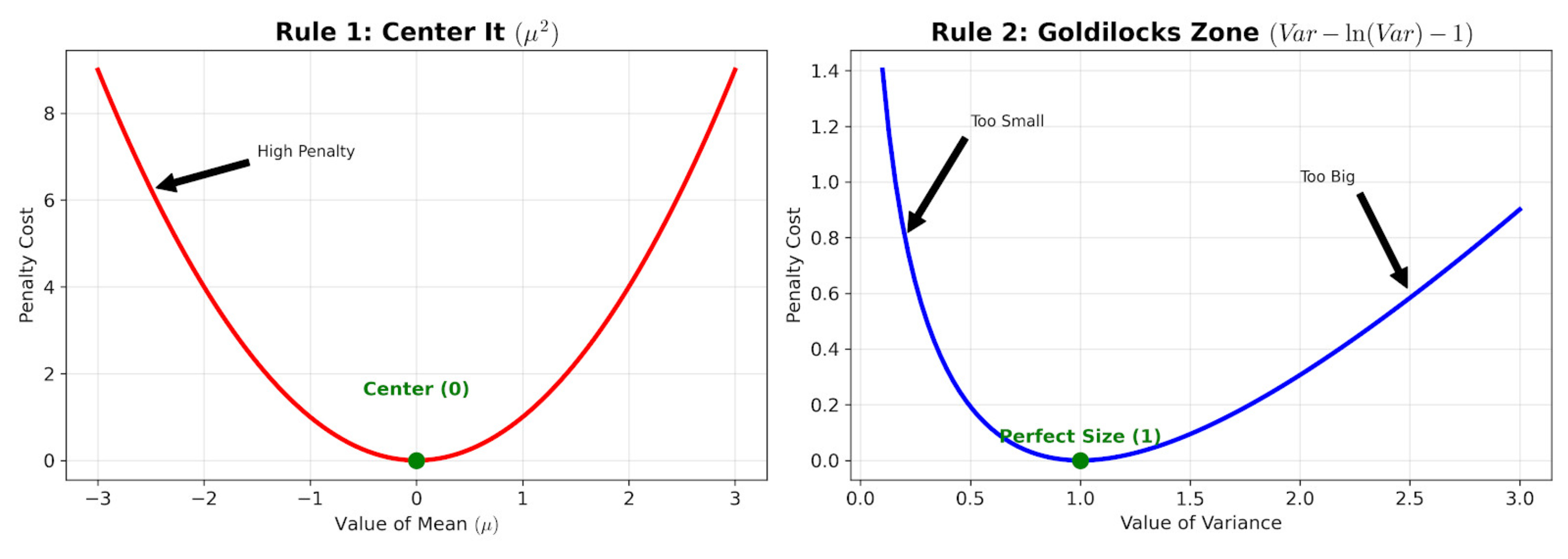
The objective of the KL divergence loss is to make sure that the latent space distribution has a mean of 0 and a standard deviation of 1.
To ensure that the mean is zero, we add a penalty if the mean deviates from zero. The penalty looks as follows:
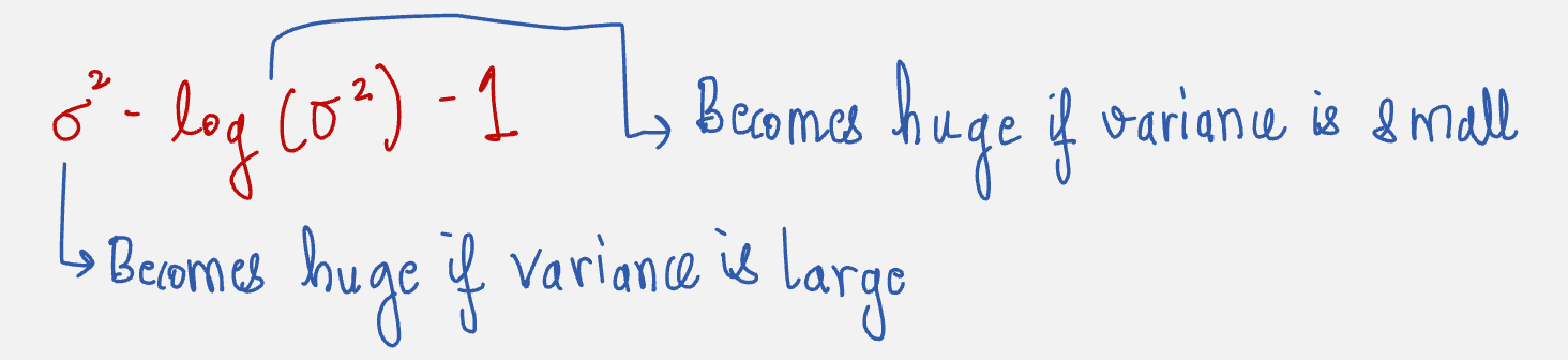
Similarly, if the standard deviation is huge, the model is penalized for being too messy. Also, if the standard deviation is tiny, then also the model is penalized for being too specific.
The Penalty looks as follows:
Here is the Google Colab Notebook which you can use for training: https://colab.research.google.com/drive/18A4ApqBHv3-1K0k8rSe2rVOQ5viNpqA8?usp=sharing
Training the VAE on MNIST Dataset:
Let us first visualize how the latent space distribution varies with the iterations. Because of the regularization term, both distributions tend to move towards the Gaussian distribution centered around the mean of 0 and the variance of 1.
When categorized according to the digits, the latent space looks as follows:
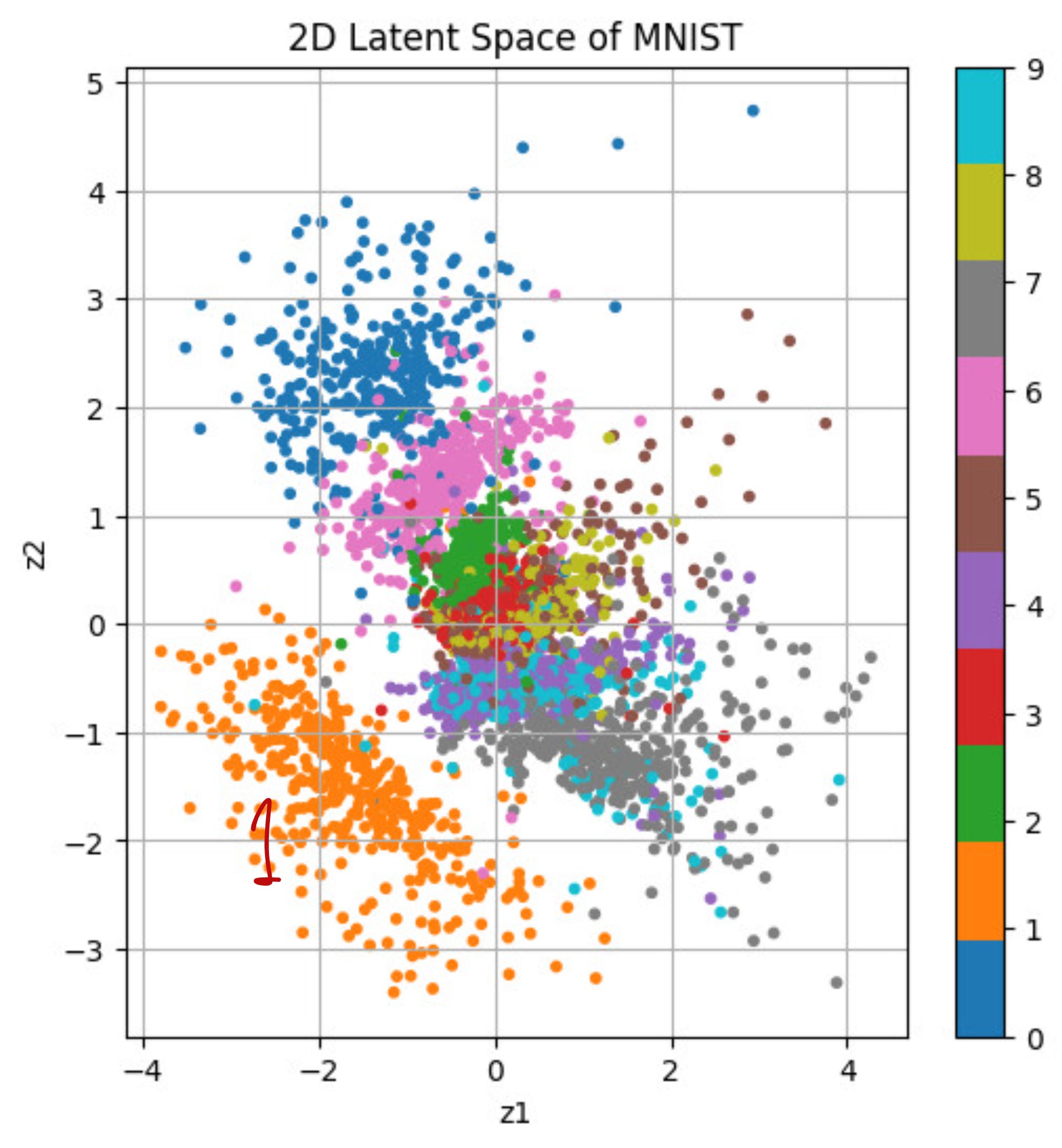
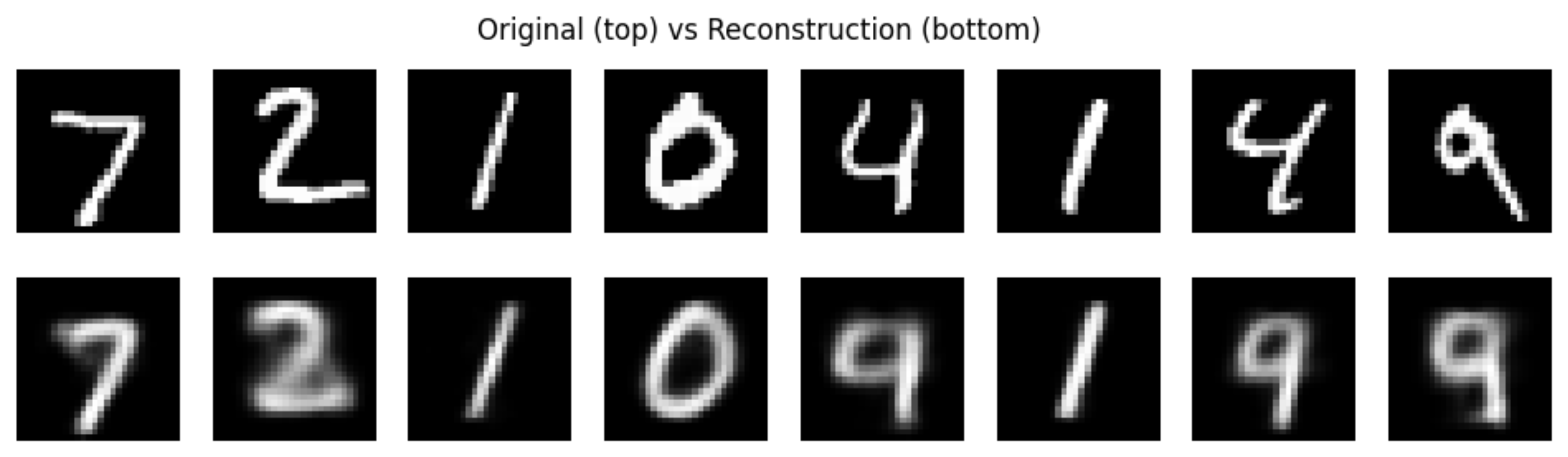
See the quality of the Reconstructions:
Sampling from the latent space:
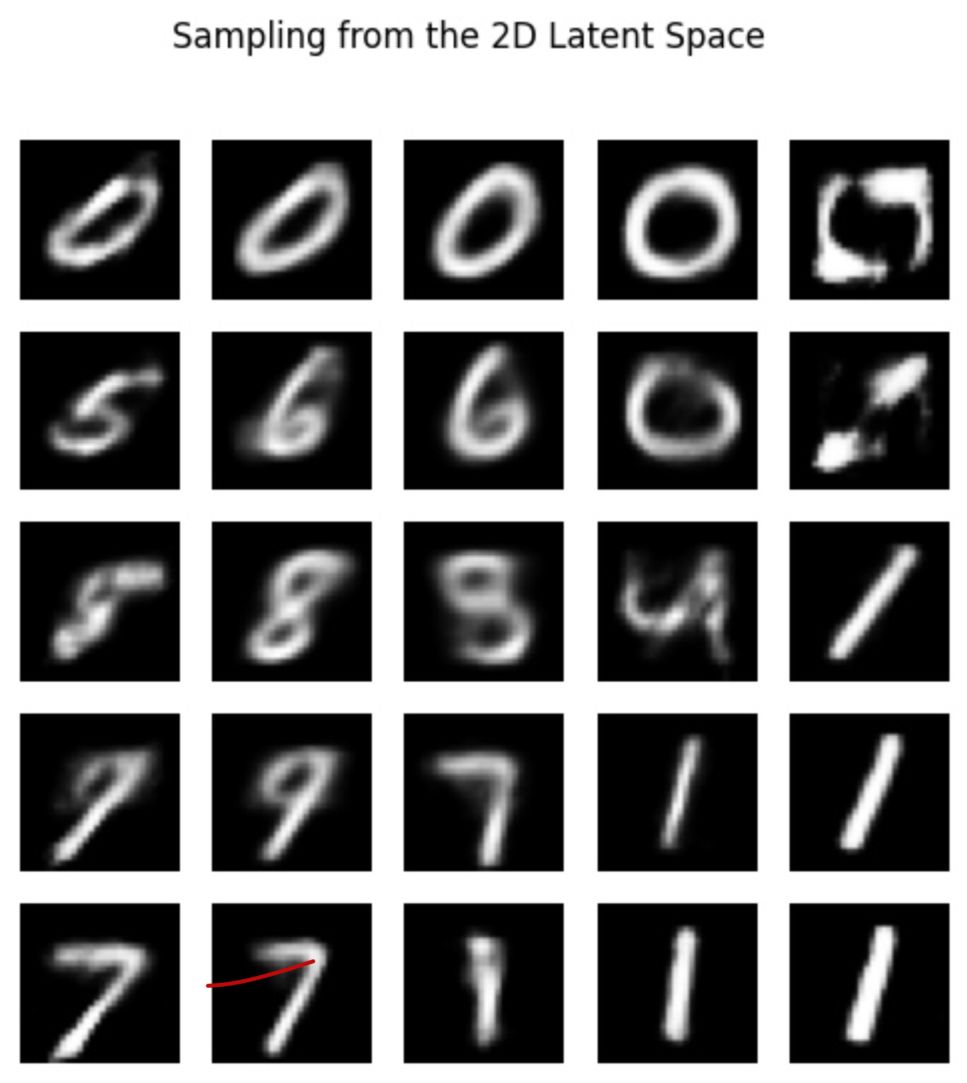
Drawbacks of Standard VAE
Despite the theoretical appeal of the VAE framework, it suffers from a critical drawback: it often produces blurry outputs.
The VAE framework poses unique challenges in the training methodology:
Because the encoder and decoder must be optimized jointly, learning becomes unstable.
Next, we will study diffusion models which effectively sidestep this central weakness.
Thanks!
If you like this content, please check out our research bootcamps on the following topics:
GenAI: https://flyvidesh.online/gen-ai-professional-bootcamp
RL: https://rlresearcherbootcamp.vizuara.ai/
SciML: https://flyvidesh.online/ml-bootcamp