
ResNet: The architecture that changed ML forever
Legendary ML paper with 250,000+ citations


The world of ML has seen many innovations since deep neural networks. However, no development has been quite as transformative as the introduction of the Residual Network (ResNet) by Microsoft in 2015.
Link to ResNet paper on arXiv: https://arxiv.org/pdf/1512.03385
This architecture did not just refine existing techniques, it opened an entire new method that inspired researchers to think differently about neural network design.
Today, ResNet is a cornerstone in state-of-the-art applications across computer vision and beyond, making it one of the most groundbreaking achievements in modern artificial intelligence.
ResNet was introduced by Kaiming He, Xiangyu Zhang, Shaoqing Ren, and Jian Sun. These researchers were working at Microsoft Research when they proposed the Residual Network architecture in 2015, which went on to achieve groundbreaking results in the ImageNet and Microsoft COCO challenges. The paper has now a mind-blowing 260k+ citations!

Vanishing gradient: Deep Learning’s greatest hurdle
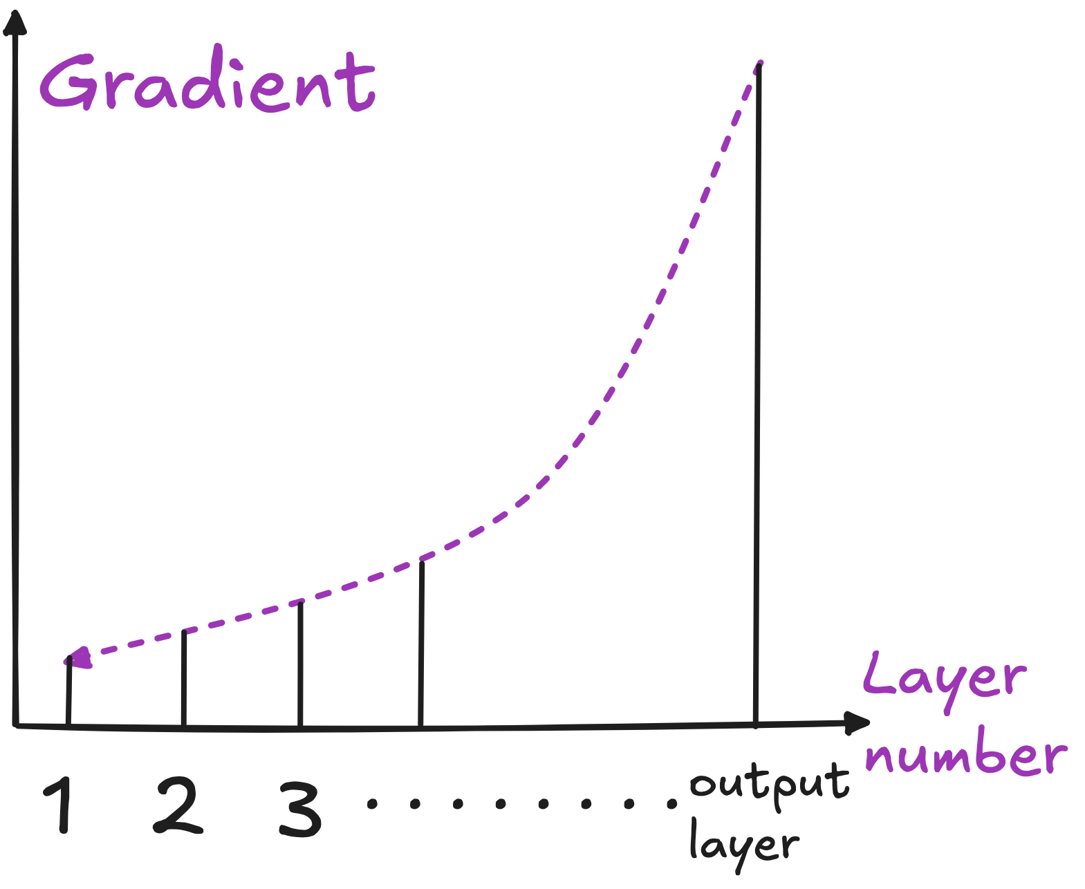
Researchers have long understood that deep neural networks possess remarkable power to learn complex patterns in large datasets. As the number of layers increases, these networks become capable of representing intricate features and relationships.
However, this complexity comes with a serious challenge: the deeper the network, the less each initial layer contributes to the final output and thus to the overall loss. In essence, when there are many layers, early layers barely affect the network’s predictions, causing their gradients (the signals used to update weights) to diminish dramatically.

When the gradient of the loss function with respect to a layer’s weights becomes very small, those weights hardly change during backpropagation. As a result, initial layers do not learn effectively, and the entire network can suffer from poor performance or fail to converge altogether. This dilemma, known as the vanishing gradient problem, stood as a major obstacle in training very deep networks.
ResNet solved vanishing gradient forever
Before ResNet, increasing a network’s depth often led to the vanishing gradient problem. Then came ResNet, bringing a simple yet profound solution.
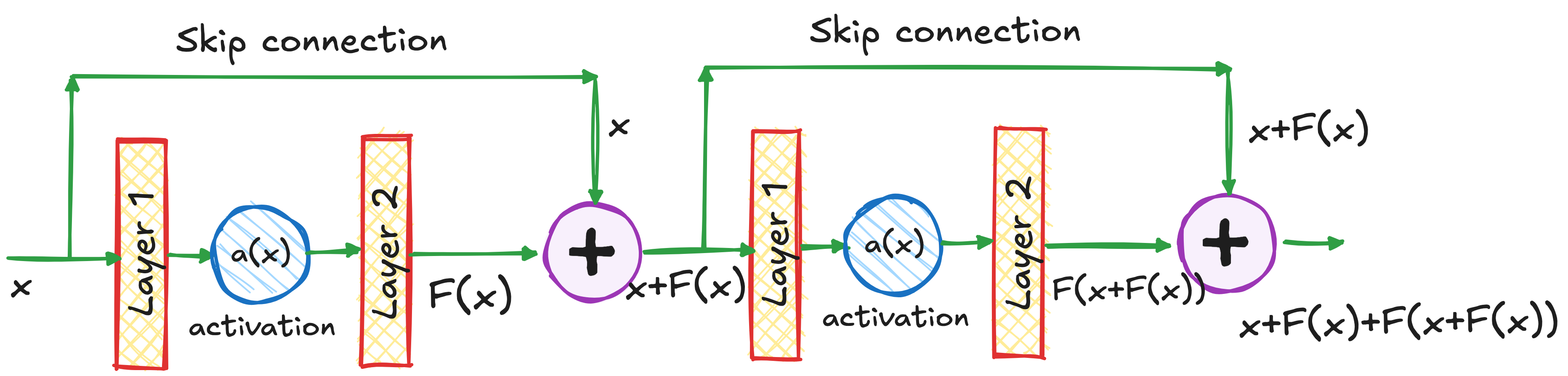
Instead of expecting each layer to learn a completely new representation, ResNet builds “residual connections” (also known as skip connections) that allow the original input to flow directly to deeper layers.
In mathematical terms, each residual block receives an input X and learns only the change needed to transform X into a better representation. Formally, it outputs X+F(X), where F(X) denotes the learned residual function.

This design ensures that early-layer activations can pass straight to the final output, preserving their influence on the network’s predictions. By allowing the gradient to flow back without getting diluted through many transformations, ResNet effectively addresses the vanishing gradient problem. As a result, even very deep networks (sometimes hundreds of layers) can be trained successfully, because initial layers still receive strong updates.

In the image above, look at how the input X is also fed directly at the output. We can repeat this for how many ever number of repeating residual connections as needed. This means the even for very deep Residual Neural Networks, the earlier layer still significantly influences the output and therefore the loss. Thus, the gradient of the loss with respect to the weights of the initial layers won’t be negligible, effectively solving the vanishing gradient problem.
Outstanding performance in 2015 competitions
Shortly after its introduction, ResNet dominated the ImageNet Large Scale Visual Recognition Challenge (ILSVRC) 2015. In the classification task, ResNet-based models achieved a top-5 error rate that surpassed all competitors. This victory signaled a major leap in performance, as it was the first time a network of such depth could outperform shallower architectures so convincingly.
In addition to the classification challenge, ResNet scored first place in the ILSVRC 2015 detection, localization, and segmentation tasks. It also delivered winning results in the Microsoft COCO detection tasks that same year. These back-to-back achievements quickly established ResNet’s reputation as a formidable architecture, influencing how future deep models would be built.
Why is residual link such a big deal?
Consider the task of improving the resolution of an image starting with a blurred image. You can train a neural network such that it directly predicts the final output, which is the high-resolution image.
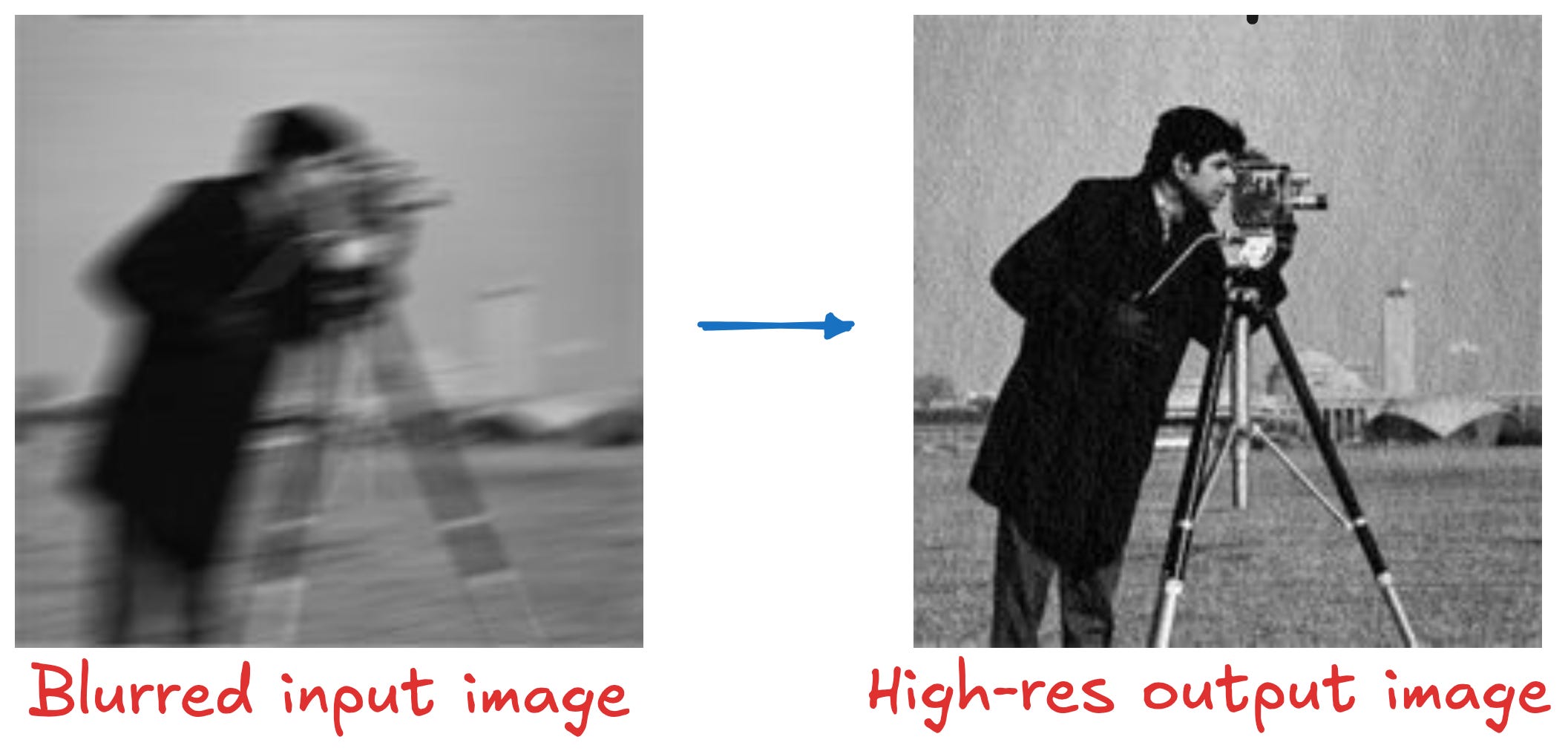
However, most of the information in the enhanced image already exists in the original image. If you were building an algorithm to transform the original image to the enhanced version, you would not want it to relearn everything from scratch. You would want it to simply figure out how to correct what is wrong.

NOTE 1: ResNet learns only the necessary change
Core idea of residual learning
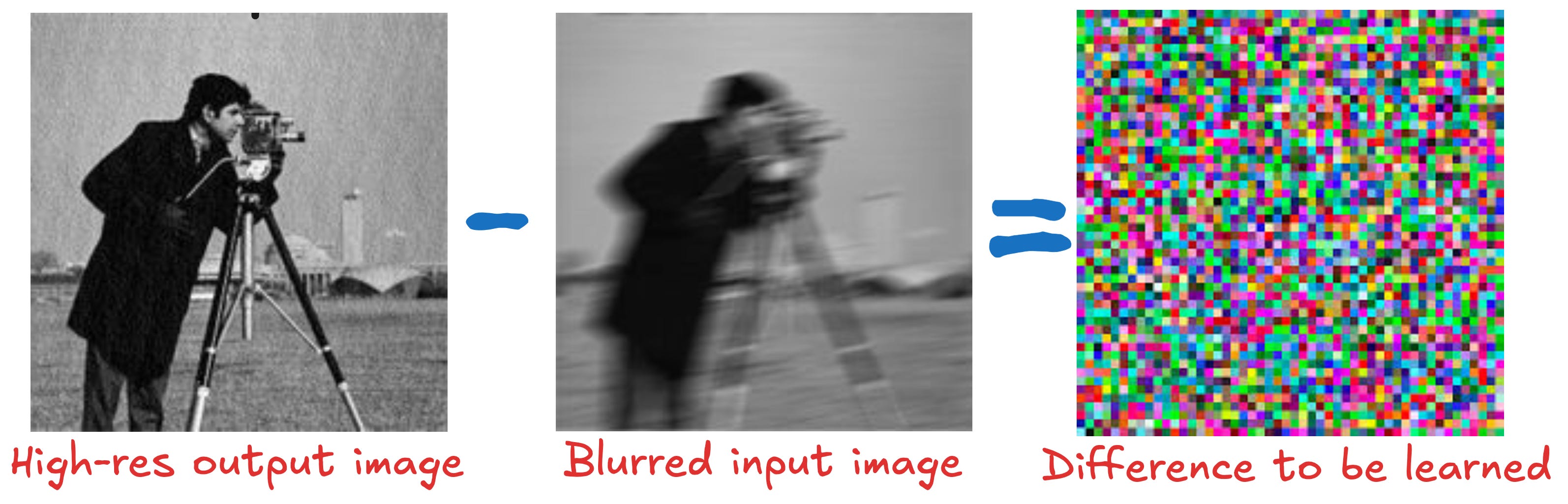
In image enhancement for example, the best approach is often to learn the difference between the original image and the enhanced image. ResNet adopts this strategy for deep neural networks. Instead of making a layer learn a complete mapping from input to output, it learns the residual or necessary adjustment.

Minimal effort, maximal effect
By focusing on the portion of the transformation that actually needs learning, the network avoids redundant computation. This also helps during backpropagation, as it keeps gradients from shrinking rapidly. This property is what allows extremely deep ResNet architectures to remain stable during training.
NOTE 2: In ResNet block, dimensions remain unchanged
In a typical ResNet block, the input and output have the same dimensions. The input passes through a few layers (for example, convolution followed by batch normalization and activation) to produce a residual transformation. Then, this residual is added back to the original input. Because the shapes match, this addition is straightforward:
Output=Input+F(Input)
The original input “skips” the main stack of layers through a direct connection, ensuring that dimension alignment is preserved. If there is a change in the number of channels between layers, a small linear projection can align dimensions, but the core principle of retaining input information remains the same.

If dimensions remain unchanged, how can you do classification?
A common point of confusion with ResNet is how it can perform tasks like classification if its residual blocks keep the same dimensions. After all, if each block preserves height, width, and number of channels, does that not suggest the network simply “enhances” the input image rather than transforming it into class scores?
In reality, while individual residual blocks typically have the same “input” and “output” dimensions to support skip connections, the overall network changes dimensions at certain stages. These changes enable feature downsampling, channel expansion, and ultimately classification. Here is how it works:
1) Residual blocks preserve dimensions only locally
Inside a standard ResNet block:
The input undergoes a few operations (like
3x3convolutions, batch normalization, ReLU) that produce an output of the same shape as the input.A skip (identity) connection bypasses those convolutions and is added to the output. This helps the network learn the residual transformation and mitigates the vanishing gradient problem.
Key point: Maintaining the same spatial dimension (height and width) and channel dimension within a block makes the skip connection straightforward. It is effectively output=input+F(input).
2) Dimension can change from one stage to another
To build a classification network, multiple residual blocks are stacked in stages. Each stage can process the feature maps at a certain resolution (for example, 56x56, then 28x28, then 14x14, etc.). At the transition between stages, ResNet uses:
Strided convolutions: A convolution layer with a stride greater than 1 (usually stride = 2) halves the spatial dimension (height and width) while often doubling the number of channels. In the example below, the stride is 3. Thus the input dimension (9x9) is reduced by a factor of 3 (3x3).

Downsample connections: If the skip path must match a changed shape, a 1x1 convolution (or a similar method) adjusts the input’s dimension so it can be added correctly.
These downsampling operations give the network a hierarchical feature representation: the early layers capture fine-grained details, while later layers focus on higher-level concepts, crucial for tasks like classification.
3) Classification through global pooling and a fully connected layer
Even though each individual block preserves local dimensions, the network as a whole significantly alters feature maps from the raw image to a condensed, abstract representation. By the final stage, the spatial dimension is typically very small, such as 7x7, and the number of channels is large (for example, 512 or 2048 channels in deeper ResNets). NOTE: An RGB image has only 3 channels. So, when I say “the final stage has 512 channels,” it means the network is producing 512 distinct feature maps (filters) at that layer. These extra channels represent a richer, more abstract representation of the image features.
Global average pooling: ResNet usually ends with a global average pooling layer that collapses the spatial dimension (e.g., 7x7) into a 1D vector by averaging across each channel.
Fully connected layer: This condensed vector then passes to a fully connected (dense) layer. The output of that layer corresponds to class scores (for example, 1,000 scores for ImageNet).
Hence, despite each residual block preserving dimensions, the overall effect of stage-by-stage downsampling and a final fully connected layer (or equivalent) makes classification possible.

ResNet as an Euler method
From a theoretical standpoint, ResNet can be viewed as an Euler method in the sense that each residual block represents a small “update” or “step” to the input:
output=input+F(input)
Comparing it to the Euler scheme for differential equations:
Translating that to ResNet’s language:
yt is like the input to the residual block.
f(yt,t) is analogous to the residual function F(Input)
The addition yt+Δt⋅f(yt,t)*yt is similar to Input+F(Input) in the ResNet block
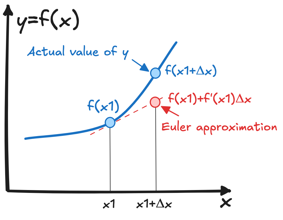
Though there is no explicit time-step parameter Δt in standard ResNets, the structure mirrors the form of iterative refinement used by the Euler method. This viewpoint suggests that each residual block is like a small “step” toward refining the representation of the data, much like taking a step in the numerical solution of a differential equation.

ResNet34 architecture
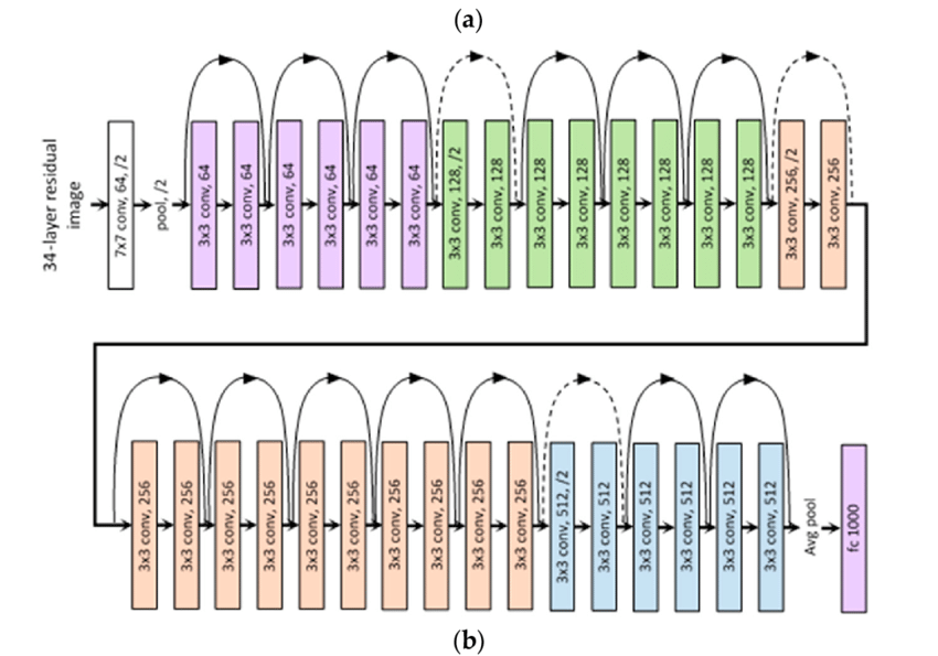
Building upon the 34-layer plain network architecture (which draws inspiration from VGG-19), ResNet introduces shortcut connections. These shortcut connections convert the plain model into a residual network, as illustrated in the figure below taken from the original 2015 ResNet paper.

When you see references such as “ResNet-50,” “ResNet-101,” or “ResNet-152,” these names indicate how many layers (or “depth”) the particular ResNet model contains. The original paper by Kaiming He et al. introduced ResNet in several depths to illustrate how their residual architecture scaled:
ResNet-18 and ResNet-34: Use basic residual blocks (two 3×3 convolutions followed by a shortcut/skip connection). These networks are relatively shallow compared to the deeper variants and have fewer parameters. They were shown to be more manageable baselines.
ResNet-50, ResNet-101, and ResNet-152: Use bottleneck blocks (three convolutions per block: a 1×1 that reduces channels, a 3×3, and another 1×1 that expands channels). The skip connection bypasses these three convolutions. This “bottleneck” structure is more parameter-efficient and helps train deeper networks while maintaining reasonable memory requirements.
What does “50,” “101,” “152” etc. mean?
A network labeled “ResNet-50” contains 50 layers that are trainable and contribute to feature transformation.
Similarly, “ResNet-101” has 101 layers, and so forth.
The jump from ResNet-50 to ResNet-101 or ResNet-152 primarily involves stacking more of these bottleneck blocks, giving the model a greater capacity to learn complex representations.
Lecture on ResNet
I have made a 45 minute lecture video on ResNet (meant even for absolute beginners) and hosted it on Vizuara’s YouTube channel. Do check this out. I hope you enjoy watching this lecture as much as I enjoyed making it.
Python implementation of ResNet for ImageNet
ImageNet is a large database of annotated images that's used to train computer vision models. It's one of the largest resources for training deep learning models for image recognition.

ImageNet as a whole contains on the order of 14 million annotated images spanning more than 20,000 categories. However, it is helpful to distinguish between:
The full ImageNet dataset: Roughly 14 million images in total, organized into tens of thousands of synsets (semantic concept classes).
The ILSVRC subset (often called “ImageNet” in practice): This is the version used for the ImageNet Large Scale Visual Recognition Challenge (ILSVRC). It has around 1.2 million training images, 50,000 validation images, and 100–150,000 test images, spread across 1,000 classes.
If someone refers simply to “ImageNet,” they are often talking about the ILSVRC 2012 (1K-class) subset. But strictly speaking, the full ImageNet dataset includes many additional categories and images, totaling around 14 million.
Install PyTorch
pip install torch torchvision pillowImports
# Import necessary libraries
import torch
import torchvision.models as models
import torchvision.transforms as T
import requests
from PIL import Image
from io import BytesIO
Downloading the Image
def download_image(url):
    """
    Download an image from the given URL with a valid
    User-Agent and return it as a PIL Image.
    """
    headers = {
        "User-Agent": (
            "Mozilla/5.0 (Windows NT 10.0; Win64; x64) "
            "AppleWebKit/537.36 (KHTML, like Gecko) "
            "Chrome/91.0.4472.124 Safari/537.36"
        )
    }

    response = requests.get(url, headers=headers)
    response.raise_for_status()  # Raises an HTTPError if the response is unsuccessful
    return Image.open(BytesIO(response.content)).convert('RGB')
Loading ImageNet labels
def load_imagenet_labels():
    """
    Download the 1,000 ImageNet class labels with a valid
    User-Agent and return them as a list indexed by class ID.
    """
    labels_url = "https://raw.githubusercontent.com/pytorch/hub/master/imagenet_classes.txt"
    headers = {
        "User-Agent": (
            "Mozilla/5.0 (Windows NT 10.0; Win64; x64) "
            "AppleWebKit/537.36 (KHTML, like Gecko) "
            "Chrome/91.0.4472.124 Safari/537.36"
        )
    }

    response = requests.get(labels_url, headers=headers)
    response.raise_for_status()
    labels_str = response.text.strip().split("\n")
    return labels_str
Preprocessing the image
def preprocess_image(image):
    """
    Transform the PIL Image into a Tensor suitable for
    the pretrained PyTorch model.
    """
    transform = T.Compose([
        T.Resize(256),             # Resize the image (shortest side = 256)
        T.CenterCrop(224),         # Crop the image at the center to 224x224
        T.ToTensor(),              # Convert the image to a PyTorch tensor
        T.Normalize(mean=[0.485, 0.456, 0.406],
                    std=[0.229, 0.224, 0.225])  # Normalize using ImageNet means and stds
    ])
    return transform(image).unsqueeze(0)  # Add a batch dimension
Classification function
def classify_image_with_resnet(image_url, topk=5):
    """
    Download an image, preprocess it, run it through
    ResNet-50, and print the top-k predictions.
    """
    # Download and preprocess
    pil_img = download_image(image_url)
    img_t = preprocess_image(pil_img)

    # Load a pretrained ResNet-50 model
    model = models.resnet50(pretrained=True)
    model.eval()  # Set model to evaluation mode

    # Disable gradient calculation for speed and memory
    with torch.no_grad():
        output = model(img_t)

    # Get label names and calculate probabilities
    labels = load_imagenet_labels()
    probabilities = torch.nn.functional.softmax(output[0], dim=0)

    # Get top-k probabilities and corresponding indices
    topk_probs, topk_indices = torch.topk(probabilities, topk)

    # Print the results
    print(f"\nImage URL: {image_url}")
    print("Top Predictions:")
    for i in range(topk):
        class_idx = topk_indices[i].item()
        prob = topk_probs[i].item()
        print(f"  {labels[class_idx]:<30} ({prob:.4f})")
Main Script
if __name__ == "__main__":
    # Replace this URL with any image URL you want to test
    test_image_url = (
        "https://images.pexels.com/photos/47547/"
        "squirrel-animal-cute-rodents-47547.jpeg?auto=compress&cs=tinysrgb&w=1260&h=750&dpr=2"
    )

    # Classify the image and print top-5 predictions
    classify_image_with_resnet(test_image_url, topk=5)