YOLO: The most exciting topic in computer vision
You Only Look Once


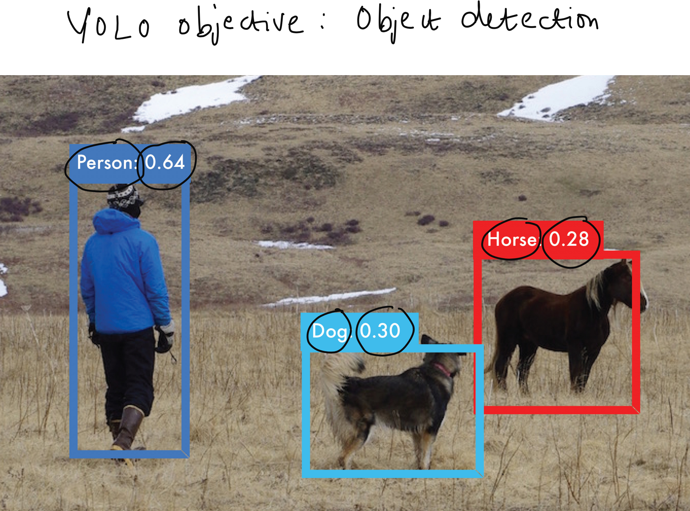
Object detection is one of the most fascinating problems in computer vision because it is not enough for the model to simply say what is in an image, it also has to say where it is. When you think about the real world, whether it is autonomous driving, security cameras, sports analytics, or even medical imaging, the “where” question is as important as the “what”. For a long time, object detection systems struggled to be both fast and accurate. The arrival of YOLO, which stands for You Only Look Once, changed that story by showing that you could have both. In this article, I want to take you step by step through how YOLO works, the questions people often ask about it, and how the family of YOLO models has evolved over the years into one of the most widely used architectures in computer vision.
The Problem Before YOLO
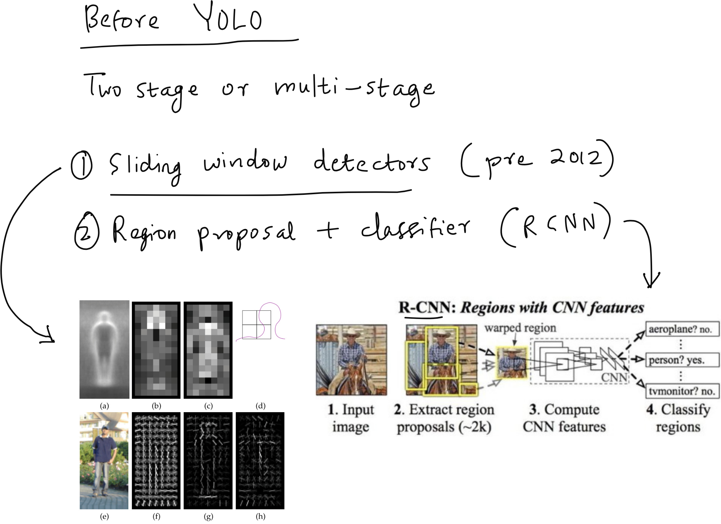
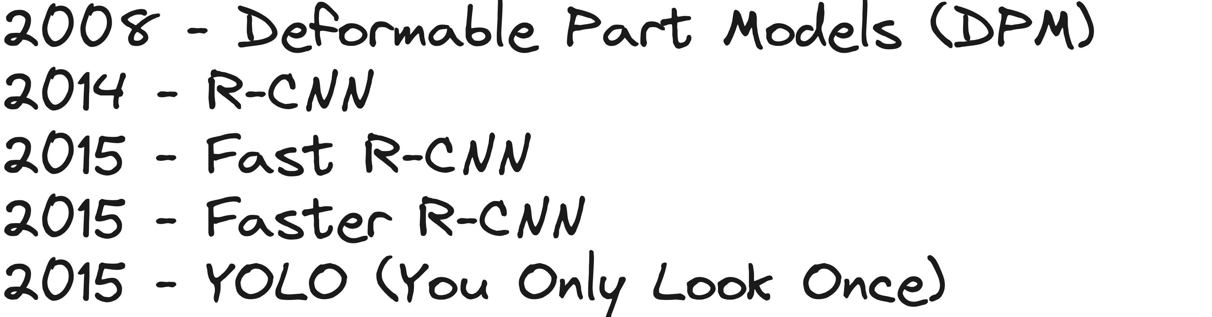
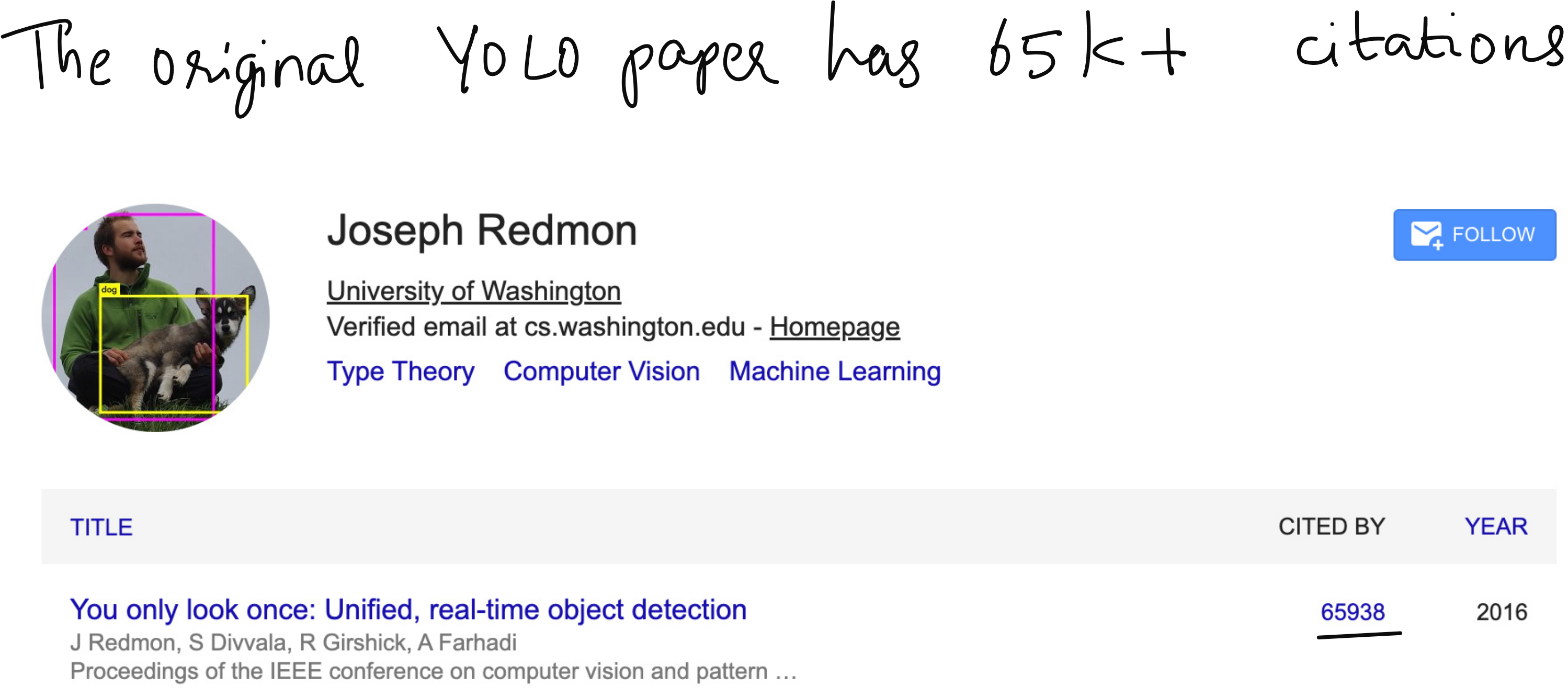
Before YOLO was introduced in 2015 by Joseph Redmon and colleagues, most object detection methods followed a region-based approach. Models such as R-CNN and its successors (Fast R-CNN, Faster R-CNN) worked by first generating region proposals, which are candidate parts of the image where an object might exist, and then running a classifier on each region. This approach was accurate, but it was slow. The model had to “look” multiple times at the image, once for each candidate region. If an image had hundreds of regions, the computational cost would go up accordingly. For real-time tasks like video analysis, this was not practical. YOLO was designed to solve exactly this bottleneck.
The Core Idea of YOLO
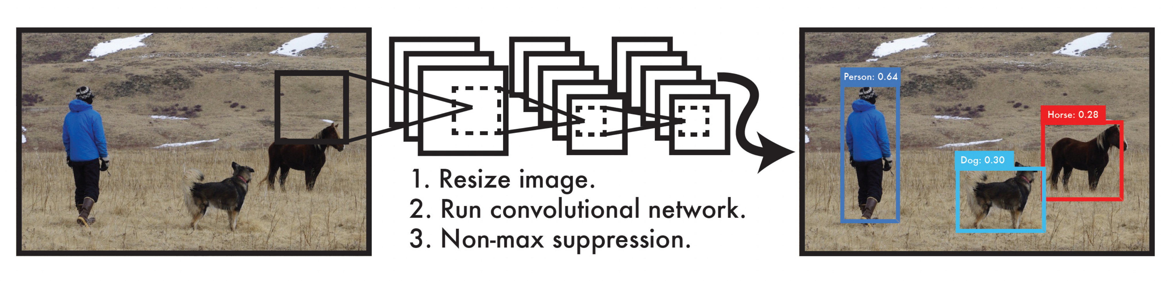
The central idea behind YOLO is very simple but extremely powerful. Instead of generating region proposals separately and then classifying them, YOLO divides the input image into a grid and directly predicts bounding boxes and class probabilities for each grid cell in a single forward pass of the network. This is why it is called You Only Look Once. You present the entire image to the network once, and the network outputs everything you need - the locations of objects, their bounding boxes, and their classes.
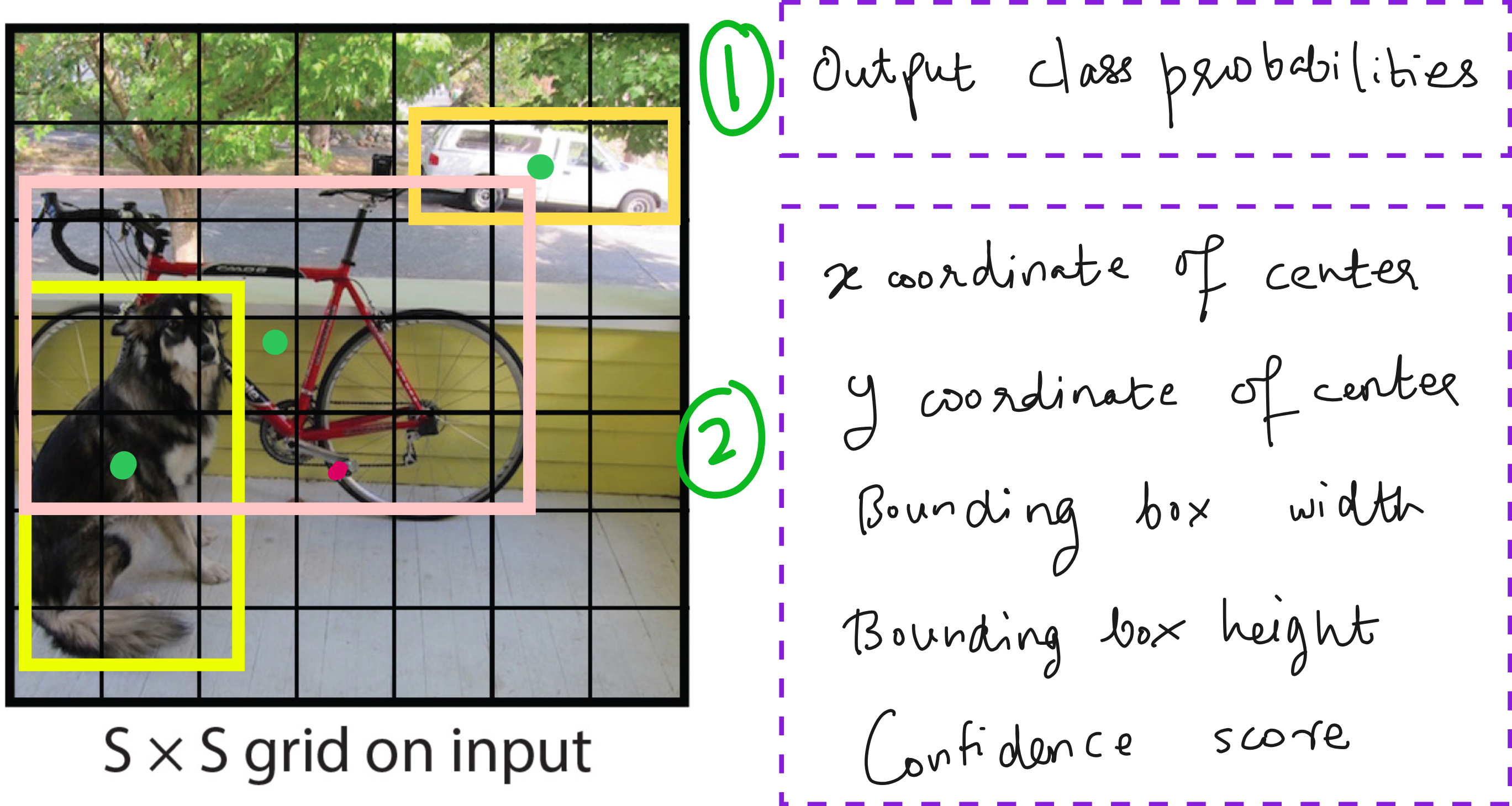
The input to YOLO is the entire image. The output is not just a single label, but a set of bounding boxes. Each bounding box is described by its center coordinates (x and y), its width and height, the class label, and a confidence score. The confidence score combines two ideas - the probability that there is an object in the bounding box and the probability that the object belongs to a particular class.
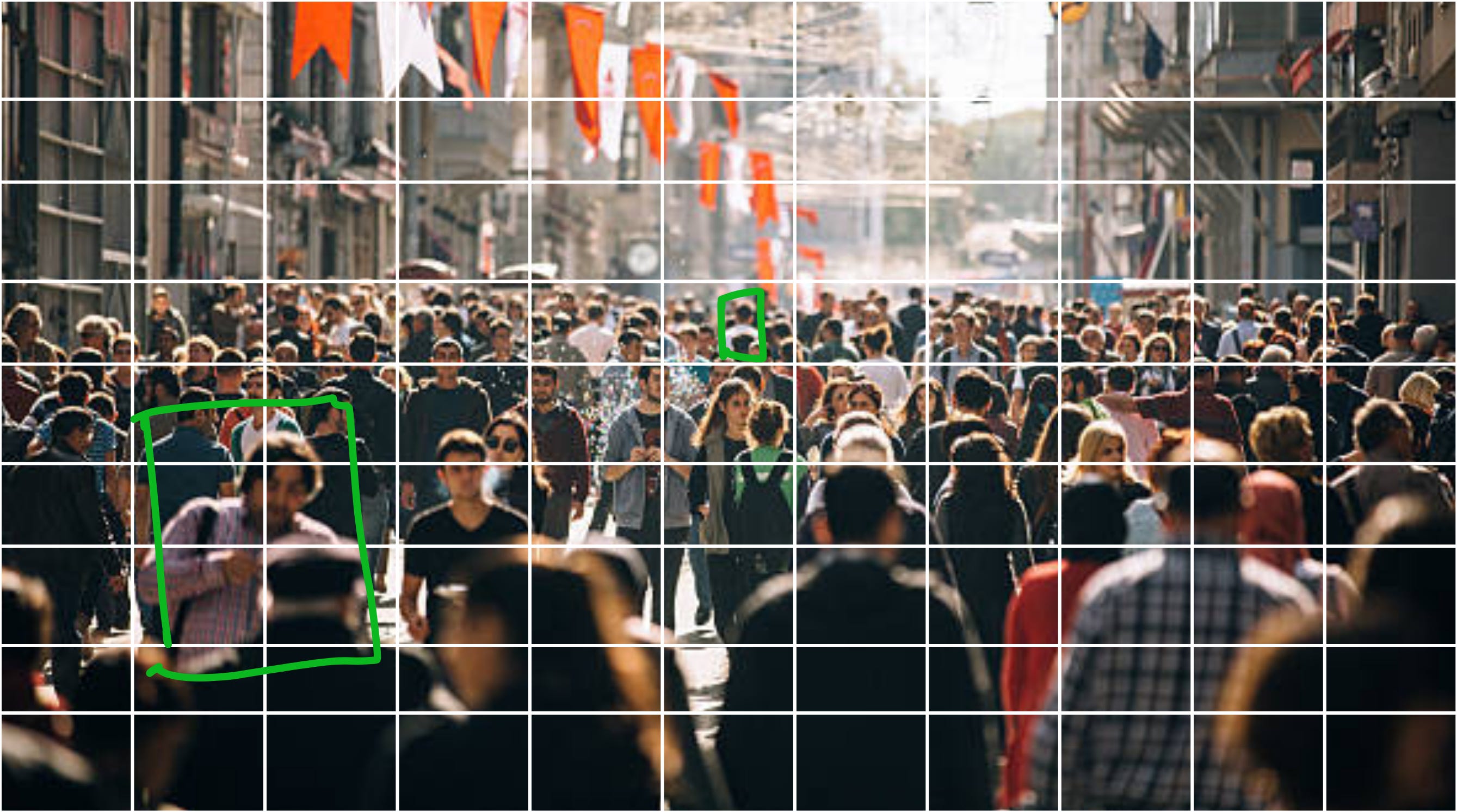
How the Image is Divided into Grids
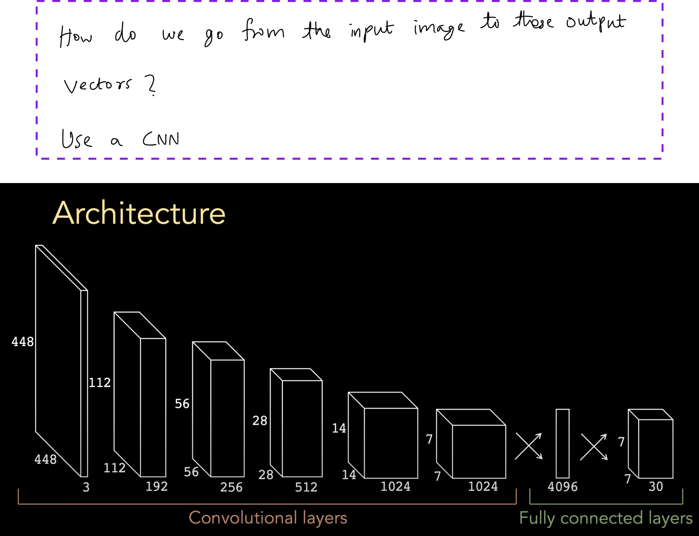
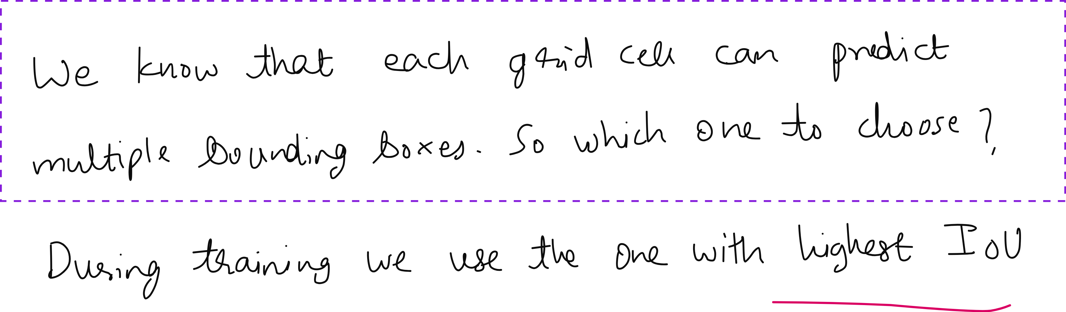
Imagine taking an image and dividing it into an S × S grid. Each grid cell is responsible for detecting objects whose centers fall inside it. For each cell, the model predicts B bounding boxes. Each bounding box includes coordinates (x, y, width, height), a confidence score, and class probabilities. So the output for one grid cell looks like a set of vectors, and the entire image output becomes an S × S × (B × 5 + number of classes) tensor.
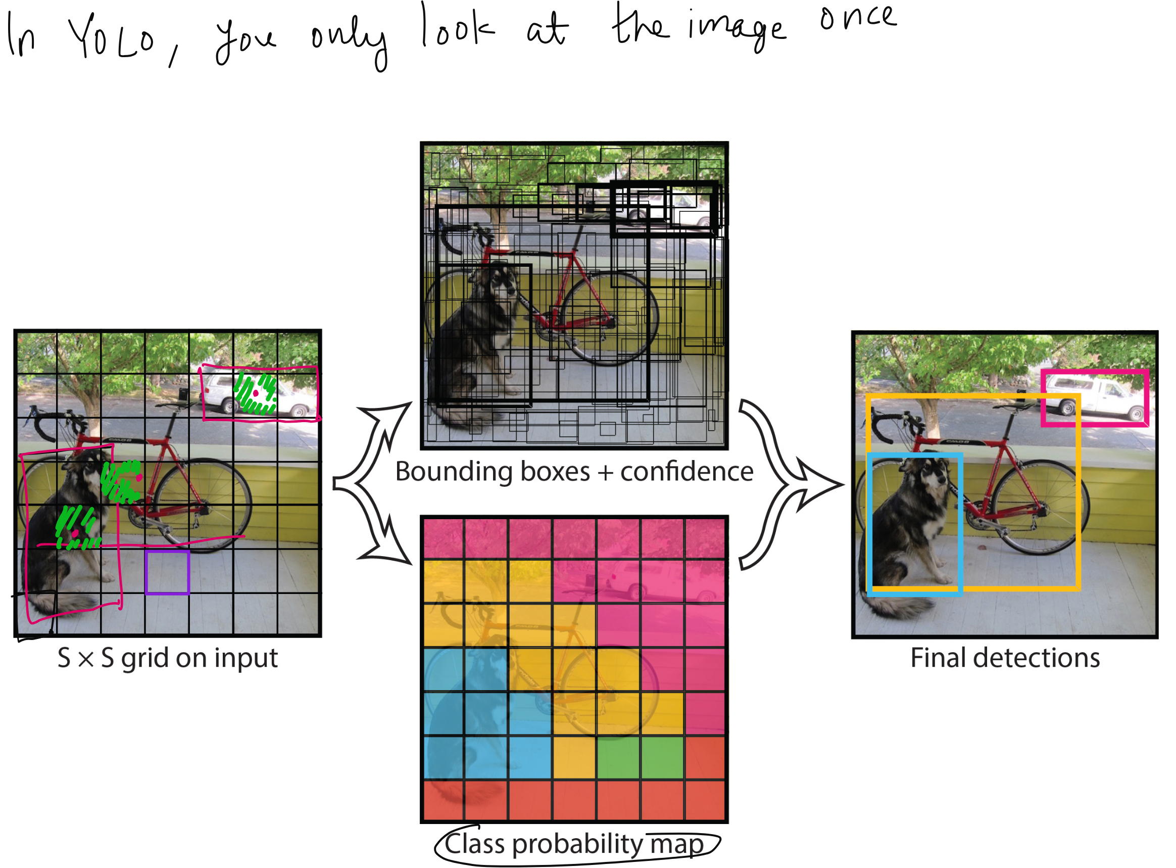
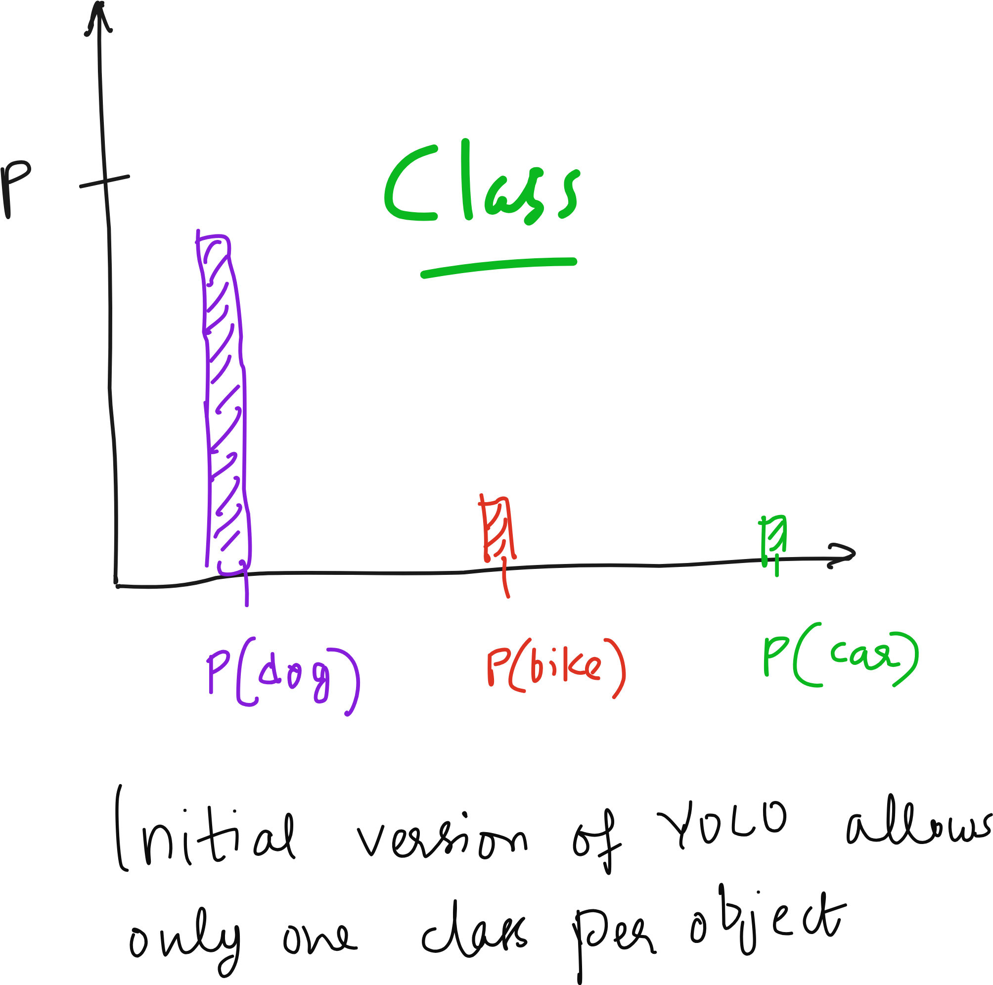
This design raises many interesting questions that often come up when teaching YOLO. For instance, what happens if two dogs are standing side by side and both fall into the same grid cell? What if an object is larger than the grid cell? Why does the bounding box sometimes appear larger than the cell itself? All of these are practical concerns, and YOLO addresses them by allowing multiple bounding boxes per cell and by learning to regress coordinates beyond the cell boundaries.
Bounding Box Predictions
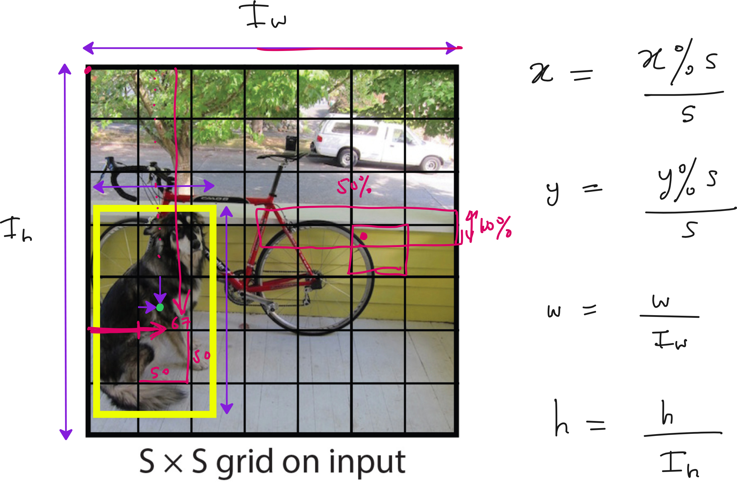
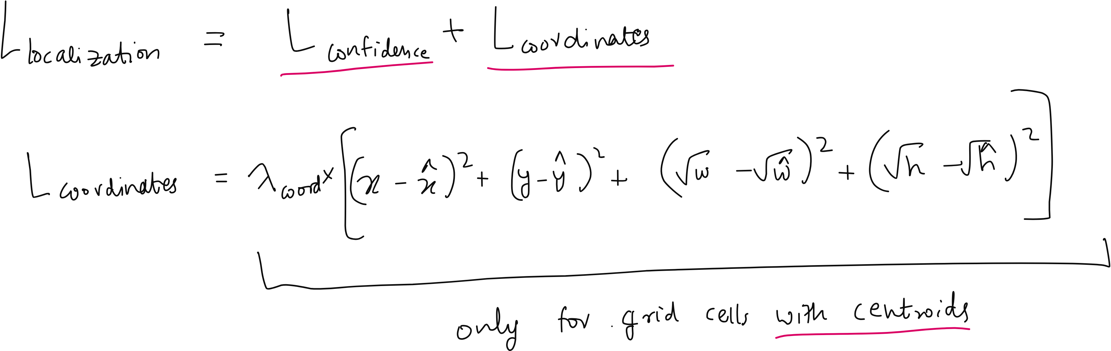
One of the most important technical contributions of YOLO is the way it parameterizes bounding boxes. The model predicts the center coordinates relative to the grid cell, and the width and height relative to the whole image size. This normalization ensures that predictions remain stable across images of different resolutions.
Another innovation was the decision to take the square root of the width and height during training. Why? Because if you make a mistake of two pixels in predicting the width of a small box, it is a much bigger problem than making the same two-pixel mistake in a large box. Taking the square root penalizes small box errors more heavily, which improves detection accuracy for small objects.
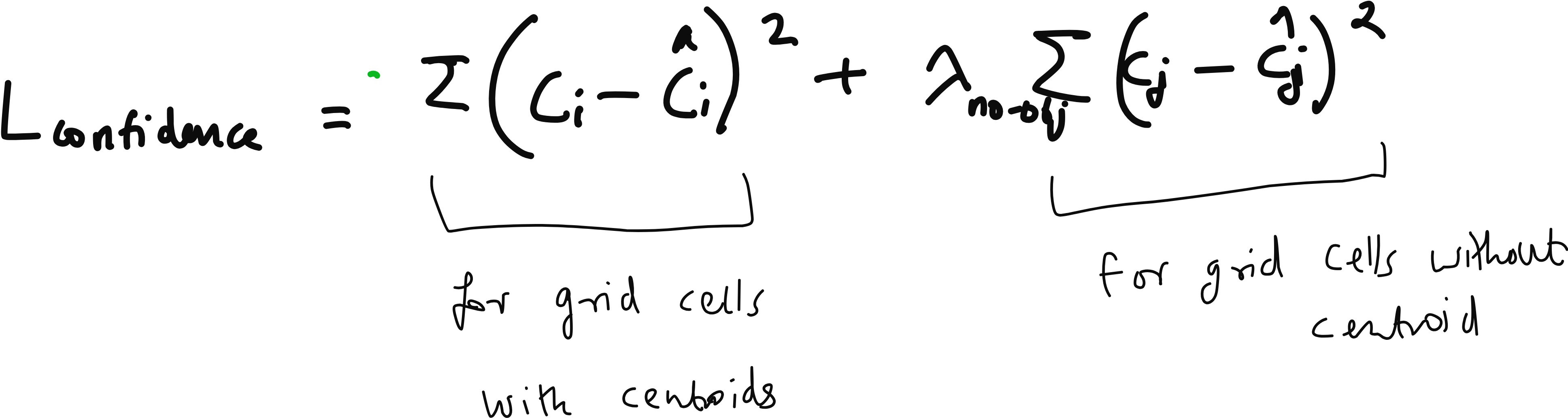
The Confidence Score and Objectness
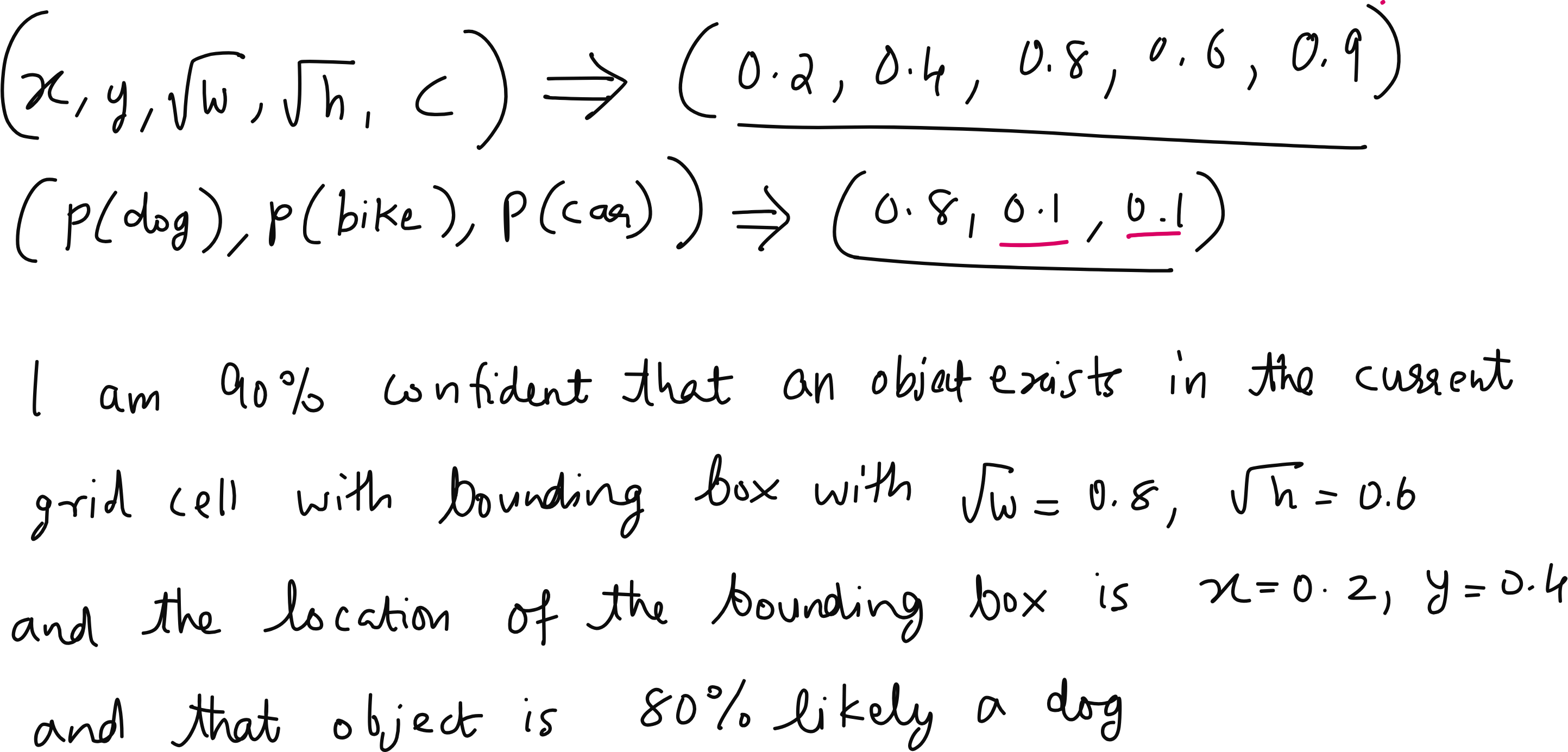
A recurring question in the discussion was about the confidence score. What exactly is it? The confidence score is the product of two terms - the probability that an object is present in the bounding box (objectness) and the probability that the object belongs to a particular class (classification). If the model is 90% sure that there is an object in the box and 80% sure that it is a dog, the confidence score is 0.72. During inference, we apply a threshold to this score to decide which detections to keep.
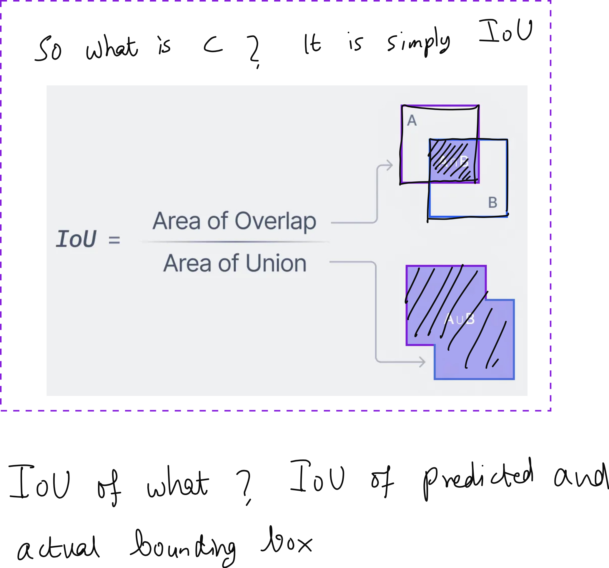
During training, the confidence score is optimized using a loss function that compares predicted boxes to ground truth boxes. The Intersection over Union (IoU) is used to measure how well the predicted box overlaps with the actual object. Low IoU is penalized in the bounding box loss.
The Loss Function
YOLO uses a multi-part loss function. It penalizes three types of mistakes:
Localization error - when the bounding box is not in the right place.
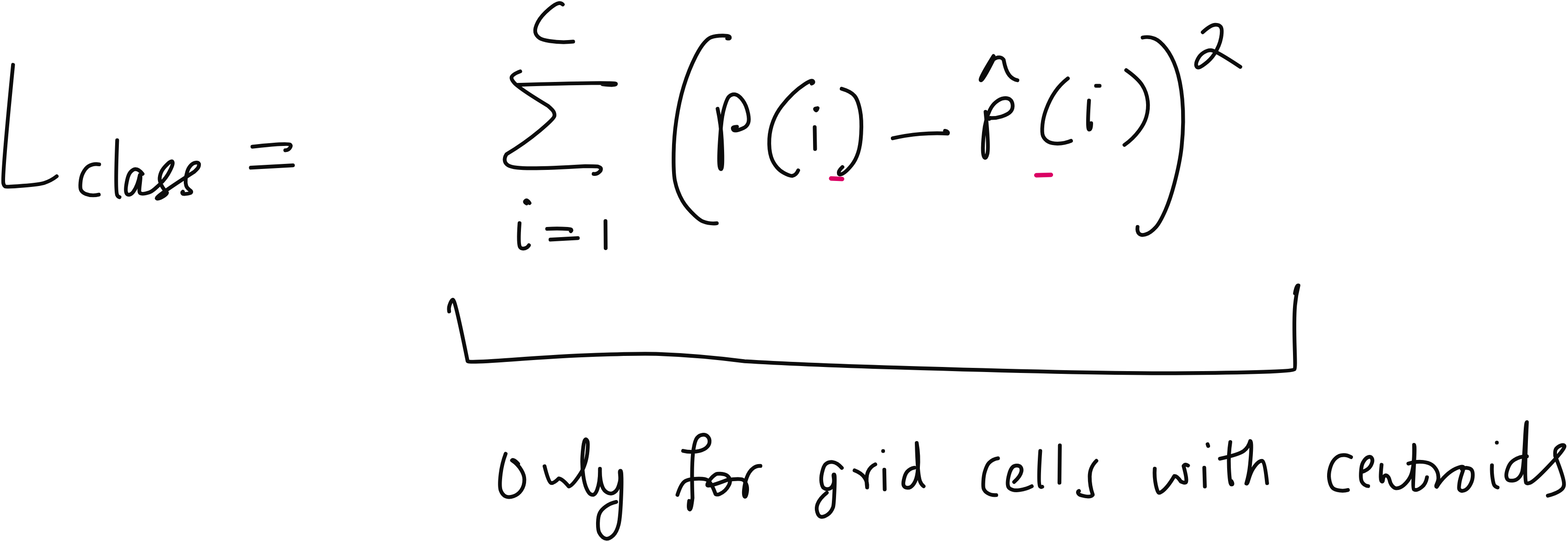
Classification error - when the class label is wrong.
Confidence error - when the model is overconfident or underconfident about the presence of an object.
In the lecture, many learners asked whether low IoU should be separately penalized or whether it is already covered in the bounding box loss. The answer is that IoU plays a central role in training and evaluation, and it is indeed captured within the loss formulation.
Training and Inference
Another set of questions was about how YOLO behaves differently during training and inference. During training, the network is presented with labeled data that includes bounding boxes and classes. The loss function guides the network to improve its predictions. During inference, the model takes an unseen image, produces bounding boxes and confidence scores, and then applies techniques such as non-maximal suppression to remove duplicate detections.
Challenges and Limitations
YOLO is not without limitations. If two objects appear in the same grid cell, the model might miss one of them. Detecting very small objects is also difficult because they may be smaller than the receptive field of the grid cell. This is why later versions of YOLO introduced anchor boxes and multi-scale detection to address these problems.
The Evolution of YOLO
YOLO has gone through many versions, each building on the previous one:
YOLOv1 (2015) - Introduced the grid-based single-pass detection framework.
YOLOv2 (2016, also called YOLO9000) - Added anchor boxes, better resolution, and could detect over 9000 classes jointly with ImageNet.
YOLOv3 (2018) - Introduced multi-scale detection using feature pyramid networks and residual connections. This improved small object detection.
YOLOv4 (2020) - Optimized training strategies, data augmentation, and backbone networks for higher accuracy while staying fast.
YOLOv5 (2020, unofficial PyTorch implementation by Ultralytics) - Became the most widely used version in practice, with improvements in usability, speed, and deployment.
YOLOv6 and YOLOv7 (2022) - Focused on industrial deployment, training efficiency, and improved accuracy on COCO.
YOLOv8 (2023, Ultralytics) - A complete rewrite, introducing a flexible framework for detection, segmentation, and classification in one.
YOLOv9 and YOLOv10 (2024) - Brought architectural changes to further push accuracy and latency trade-offs.
YOLOv11 (2024) - The latest, still being actively discussed, with a more modular architecture, better handling of small objects, and improved training pipelines.
This progression shows how YOLO started as a bold idea and has now become an entire family of models that balance speed and accuracy for diverse use cases.
Why YOLO Still Matters
YOLO is not just a technical innovation, it is a way of thinking. It showed the community that you could reformulate an entire problem in a simpler way and achieve results that were both practical and powerful. Even today, in an era where transformer-based models like DETR and RF-DETR are gaining popularity, YOLO continues to be widely used because it is efficient, robust, and battle-tested in real-world applications.
Conclusion
When we teach YOLO, the questions that come from learners are very revealing. At first, they want to know what a bounding box is, what a class score is, and how confidence is measured. Slowly, they start asking about anchor boxes, IoU, loss functions, and comparisons with other models. This journey mirrors the journey of the field itself, where a simple but bold idea grew into a family of models that define the state of the art in object detection.
If you step back and reflect, YOLO is a reminder that in computer vision, as in life, sometimes it is better not to keep looking again and again, but to look once, look carefully, and then act decisively.