What exactly is a VLM (Vision-Language Model)?

How does it work and how can you build one from scratch?

Table of contents

1. What is a VLM?

2. How do VLMs work?

   1. Visual encoder

   2. Text encoder

   3. Multimodal fusion module

      1. Early fusion

      2. Late fusion

      3. Cross-attention fusion

3. Some popular VLMs

4. Questions that can come up during VLM design

5. Let us start with the simplest idea: Dual encoder

6. Understanding contrastive learning

7. Contrastive loss formula

8. Contrastive Language-Image Pre-training (CLIP)

9. Let us build a VLM

   1. Task description

   2. Dataset

   3. Model architecture

   4. Image encoder

   5. Text encoder

   6. Loss function

10. Embedding similarity before and after training

11. Why is this model called “nano”?

    1. Image Encoder: Number of parameters

    2. Text Encoder: Number of parameters

12. Conclusion

13. Relevant resources

What is a VLM?

VLMs are AI models that can understand both images and text together.

VLMs can take both text and image as input whereas LLMs by default only take text input. So what is the output produced by a VLM? Output is whatever we design it to be. But our goal is to “align” the visual and textual representation in VLMs.

You may have heard of this in the context of the term “multimodal alignment” - alignment of different modalities.

Let us try to understand with a simple example. If I write “apple” or if I say the word “apple” or if I show you the picture of an apple, they all represent the same thing or the same idea. Somehow your brain represents all these 3 modalities (text, sound, picture of apple) with some sort of alignment.

If I write “apple” or if I say the word “apple” or if I show you the picture of an apple, they all represent the same thing or the same idea.

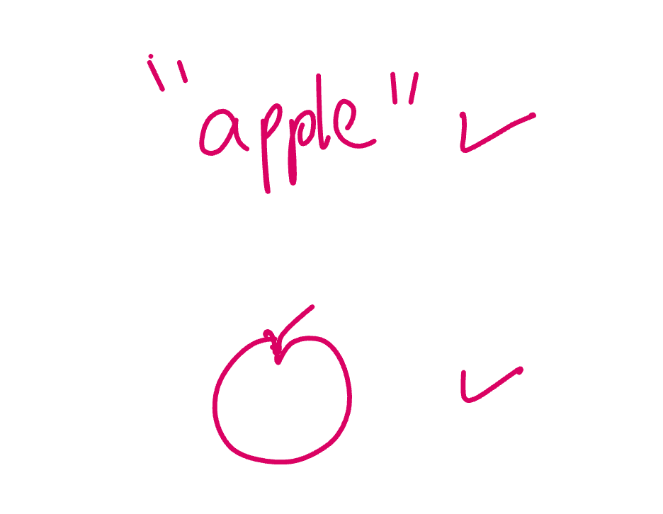
LLMs represent text or tokens using vectors - called embeddings. VLMs also do that same because they are an extension of LLMs.

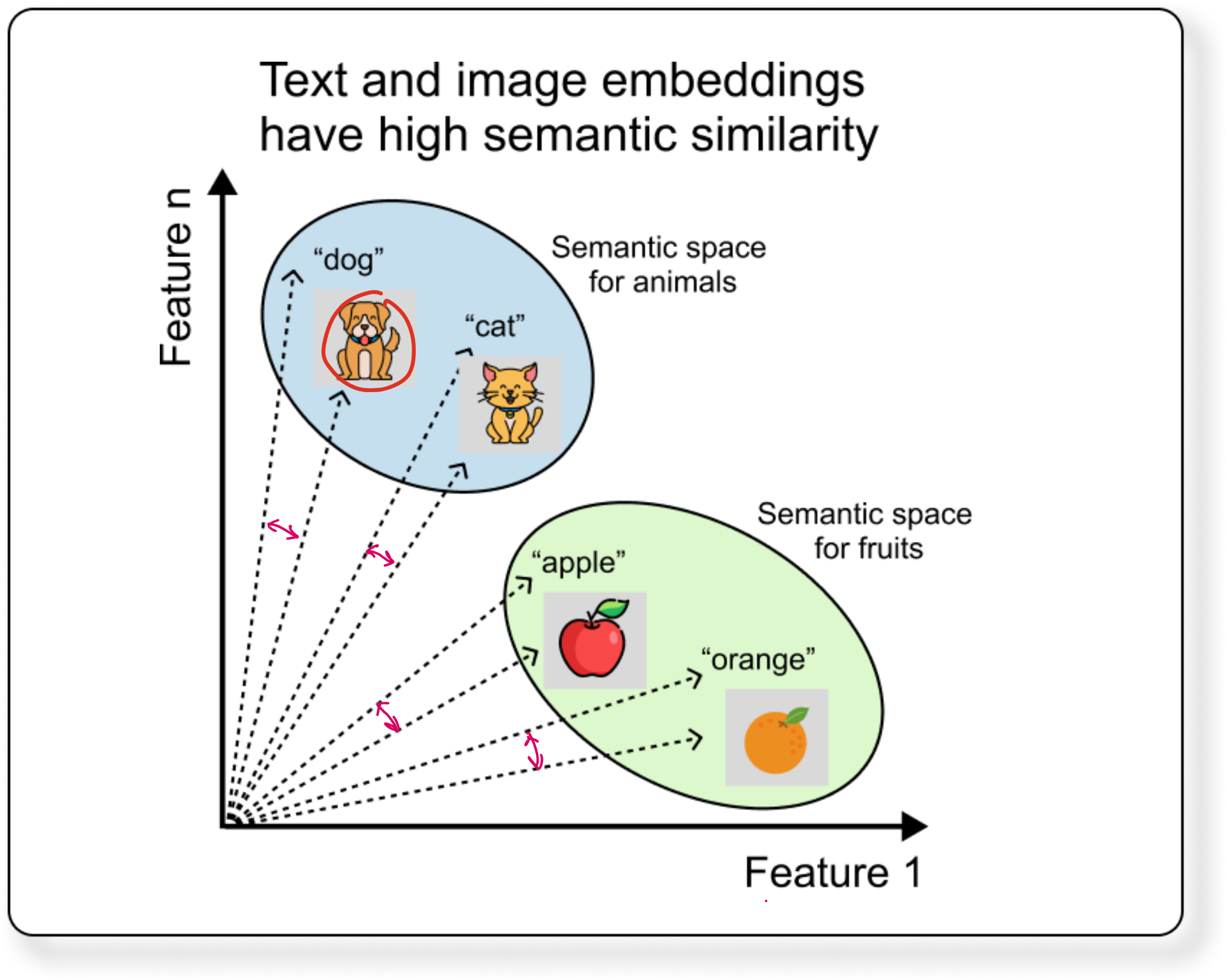
The basic idea of VLM is that the text and image embeddings (or vectors) that represent same thing should have high similarity. A simple mathematical representation of similarity between 2 vectors is the cosine of the angle between then. If the vectors are perfectly parallel, the cosine similarity will be 1.

The basic idea of VLM is that the text and image embeddings (or vectors) that represent same thing should have high similarity

If we take a step back to what models could do before VLMs, we can see that models could take care of either text or image. But not both.

Computer vision models like CNNs or Vision Transformers handle images, while language models like GPT handle text.

Computer vision models like CNNs or Vision Transformers handle images, while language models like GPT handle text.

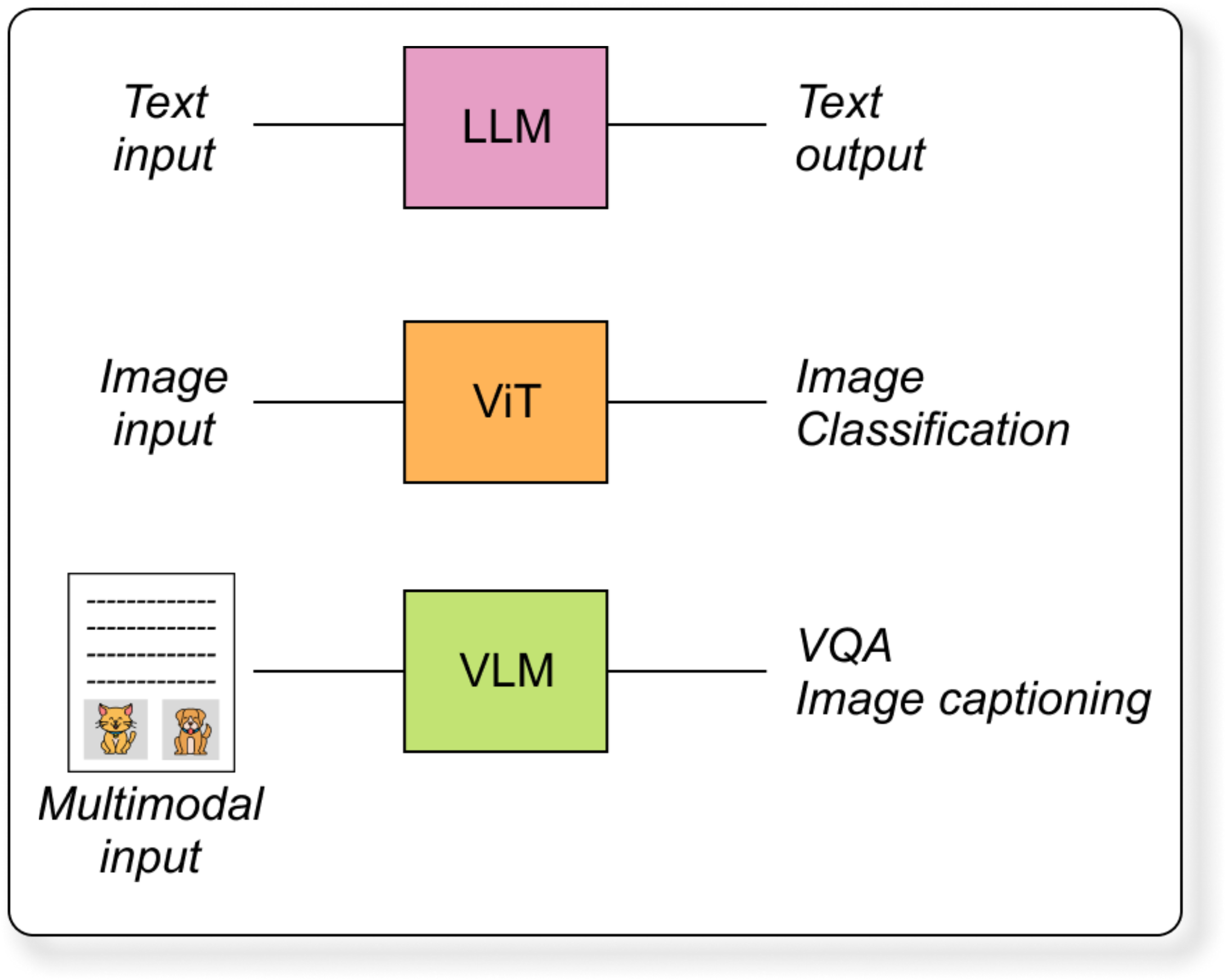
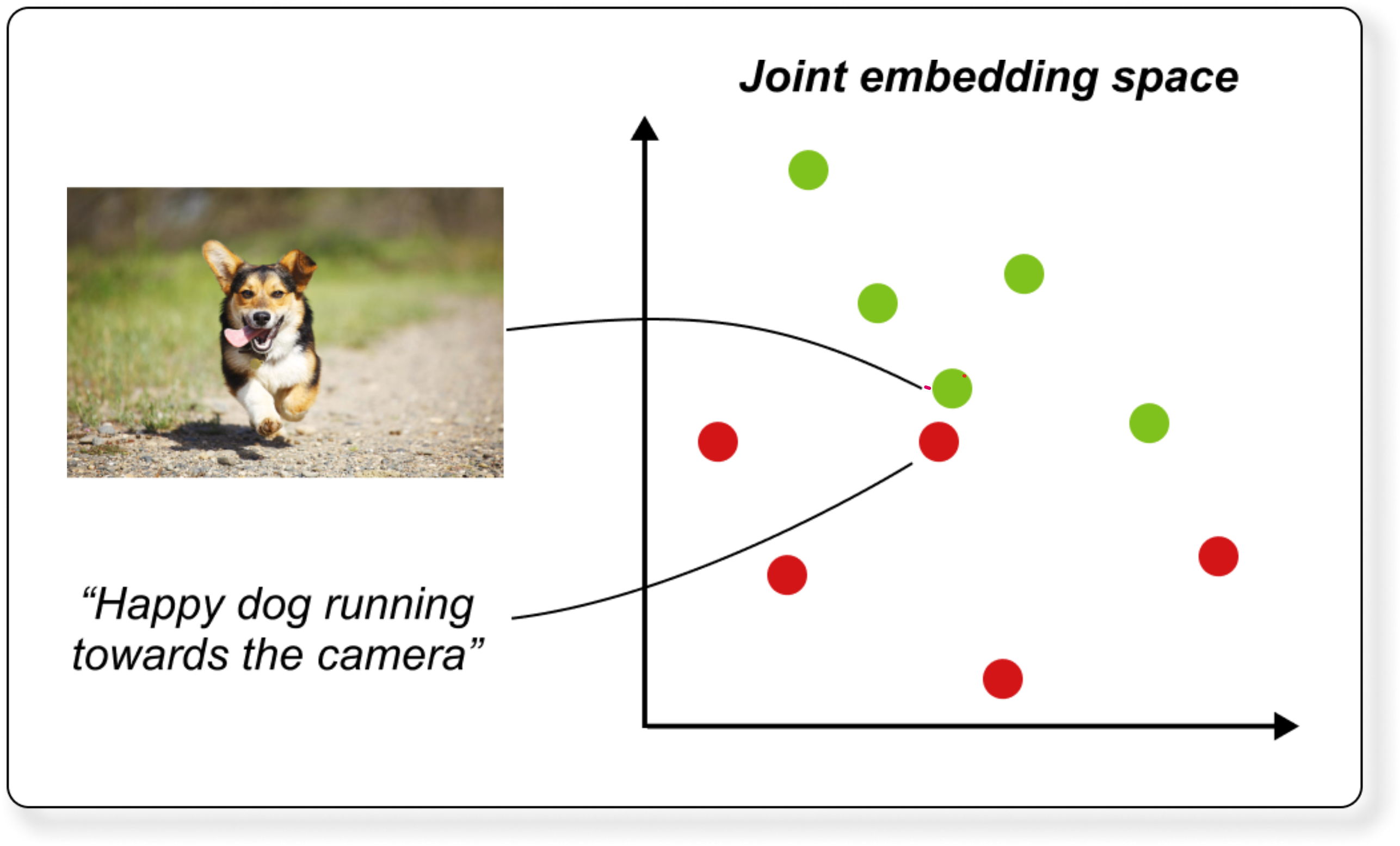
VLM bridges these two domains. It takes visual inputs (like images or videos) and text inputs (like captions, questions, or prompts) and learns a joint representation.

VLM takes visual inputs (like images or videos) and text inputs (like captions, questions, or prompts) and learns a joint representation.

Real world information is multimodal. We understand our surroundings by seeing, reading, and listening at the same time. VLM allows applications such as:

• Generating image captions automatically

• Searching for images by describing them in words

• Understanding memes, advertisements, or infographics

• Supporting robotics and self-driving systems that must interpret surroundings and follow instructions

How do VLMs work?

A typical VLM has three major components:

1. Visual encoder

Usually a Vision Transformer (ViT) or CNN, which converts the input image into a sequence of visual embeddings. Each embedding represents a patch or region of the image.

2. Text encoder

Often a Transformer-based model (like BERT or GPT), which converts the input text into language embeddings that capture the meaning of words and their context.

3. Multimodal Fusion Module

This is where the two modalities meet. There are three main ways this fusion is done.

Early fusion

Combine visual and text embeddings at the beginning and train a single transformer to process both.

Late fusion

Encode each modality separately and align them using similarity losses (e.g., CLIP).

Cross-attention fusion

Use attention mechanisms where image tokens attend to text tokens and vice versa (e.g., BLIP, Flamingo).

A typical VLM has three major components. 1) Visual or image encoder, 2) text encoder and 3) Multimodal fusion module

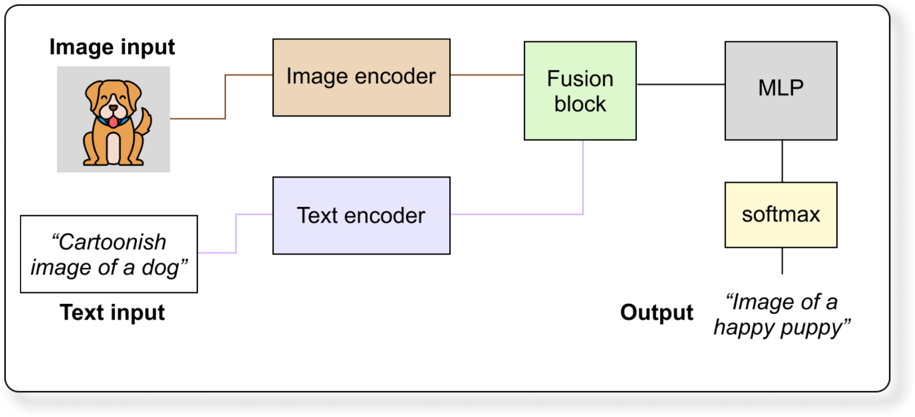
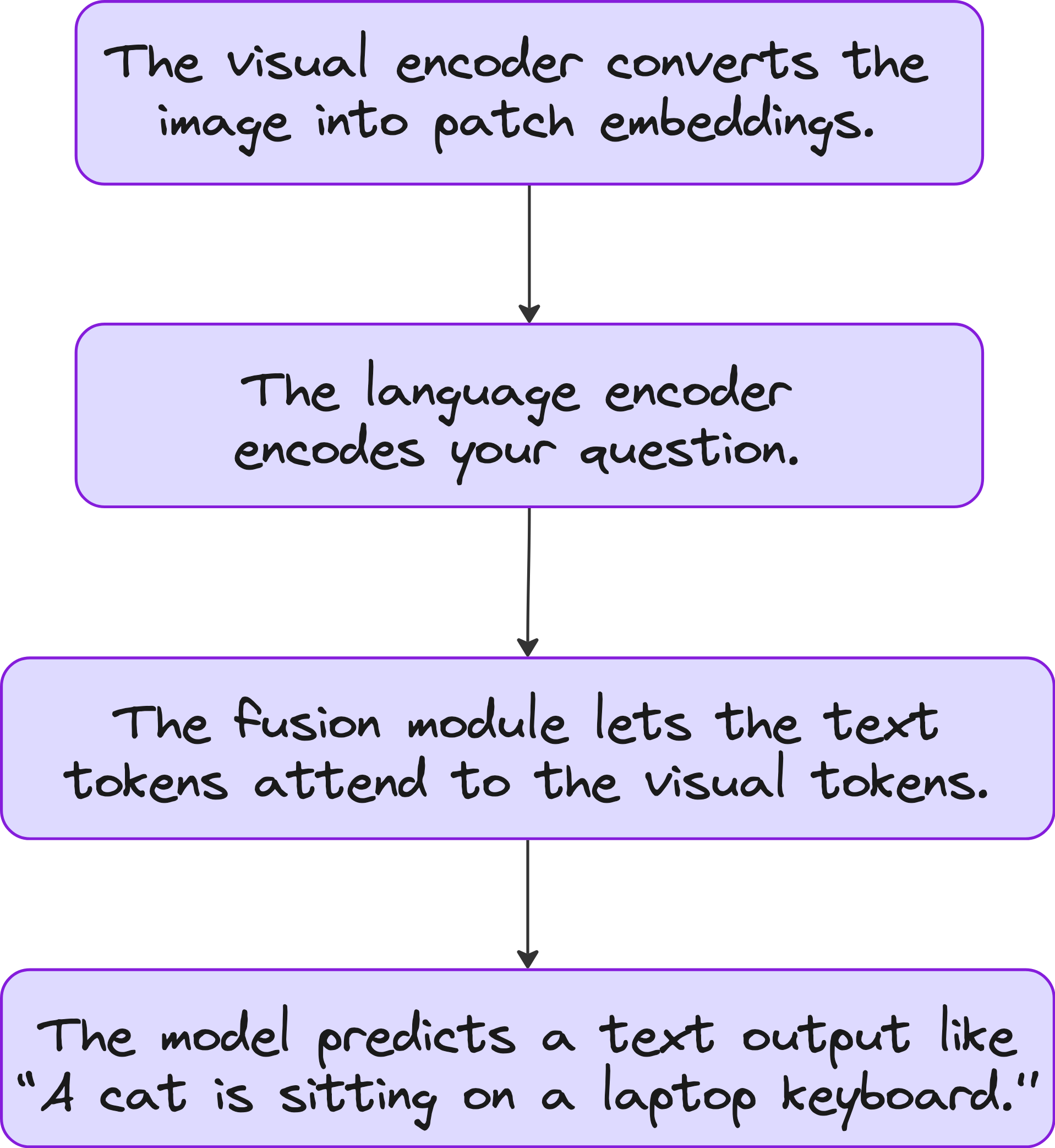
Let us see an example VLM workflow.

Suppose you input an image of a cat sitting on a laptop and a text prompt “What is happening in the image?”

Example of VLM workflow.

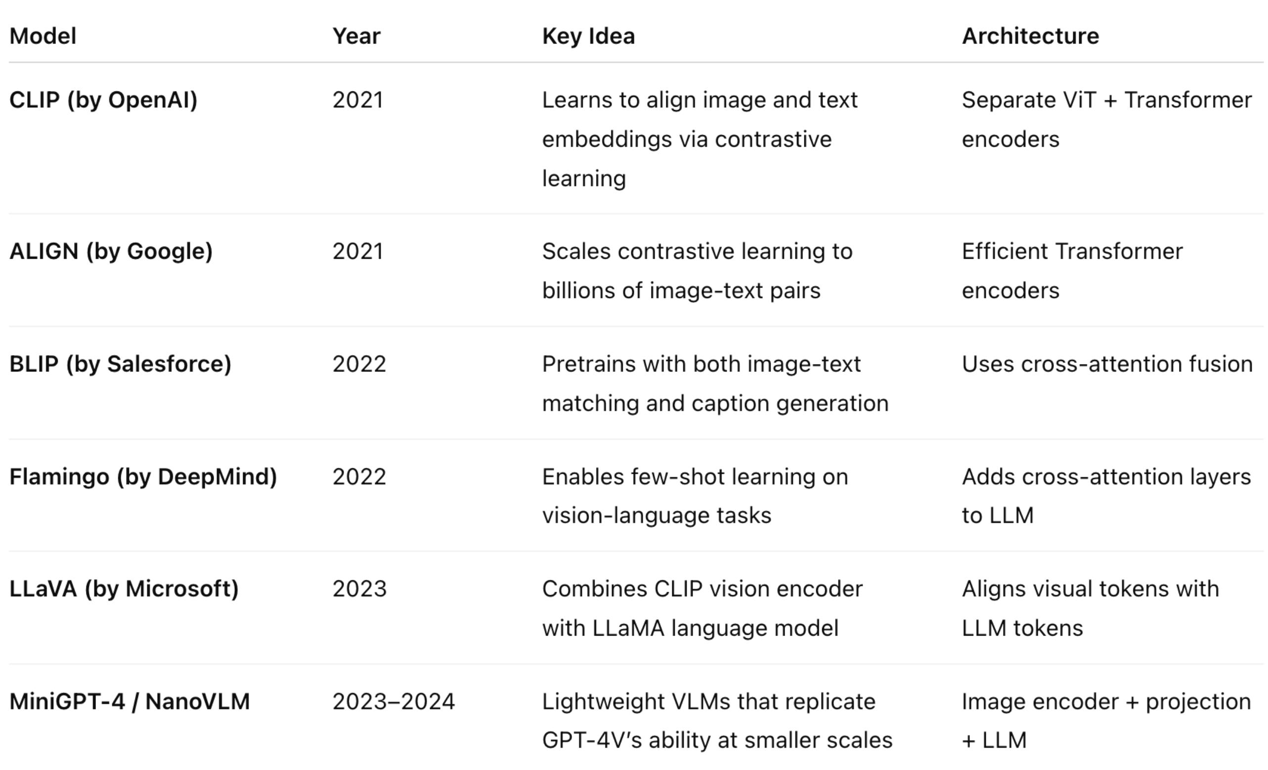
Some popular VLMs

Here are some popular VLMs that you should care about. At Vizuara we have conducted detailed lectures on a bunch of these models. Links are provided at the end of this article.

CLIP, BLIP, ALIGN, Flamingo and LLaVa are the most famous VLMs at the moment.

Questions that can come up during VLM design

Now let’s say we want to design out own VLM that can understand language and vision, there are some questions that naturally popup in our mind.

1. How to encode different modalities?

2. How to combine these modalities?

3. What kind of loss function to use?

4. Should we train from scratch or use pretrained models?

5. What type of data for training?

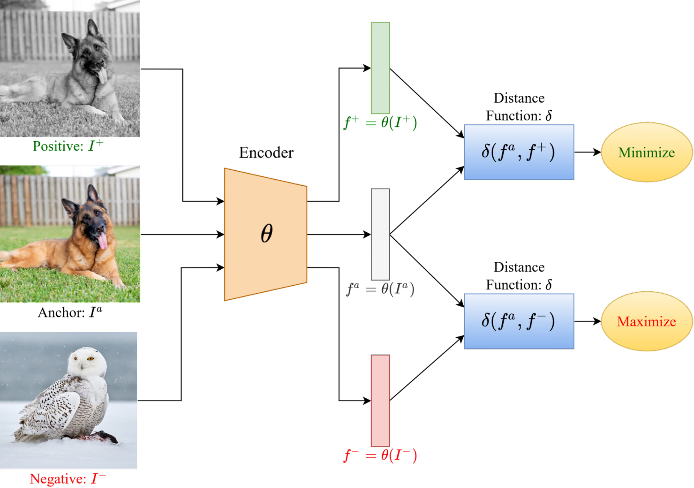
Let us start with the simplest idea: Dual encoder

Dual encoder is literally the simplest VLM.

• It has two separate encoders

• Each encoder converts its input into a vector embedding.

• Both embeddings lie in a shared feature space, so related image-text pairs have similar vectors.

• The model is trained using a contrastive loss (for example, CLIP loss) that brings matching pairs closer and pushes non-matching pairs apart. (What is contrastive learning? We will discuss in the next section)

Dual encoder has two separate encoders. Each encoder converts its input into a vector embedding. Both embeddings lie in a shared feature space, so related image-text pairs have similar vectors.

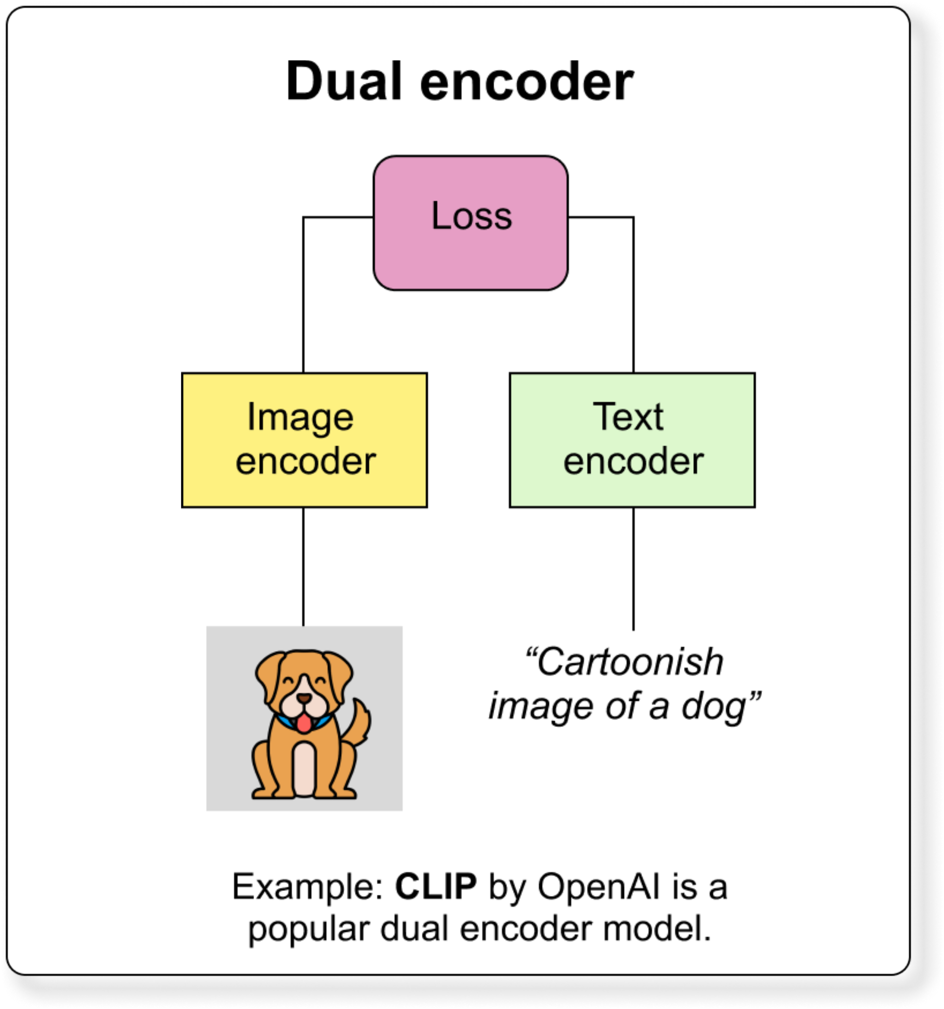
• Image Encoder is usually a CNN or Vision Transformer (ViT).

• Text Encoder is usually a Transformer (like BERT or GPT).

• It is mainly used for image-text retrieval, zero-shot classification, and multimodal alignment.

• Because encoders are independent, embeddings can be pre-computed, making it fast and scalable for large datasets - you don’t have to recalculate for each search query.

Now before we proceed ahead, we should understand what exactly is contrastive learning.

Understanding contrastive learning

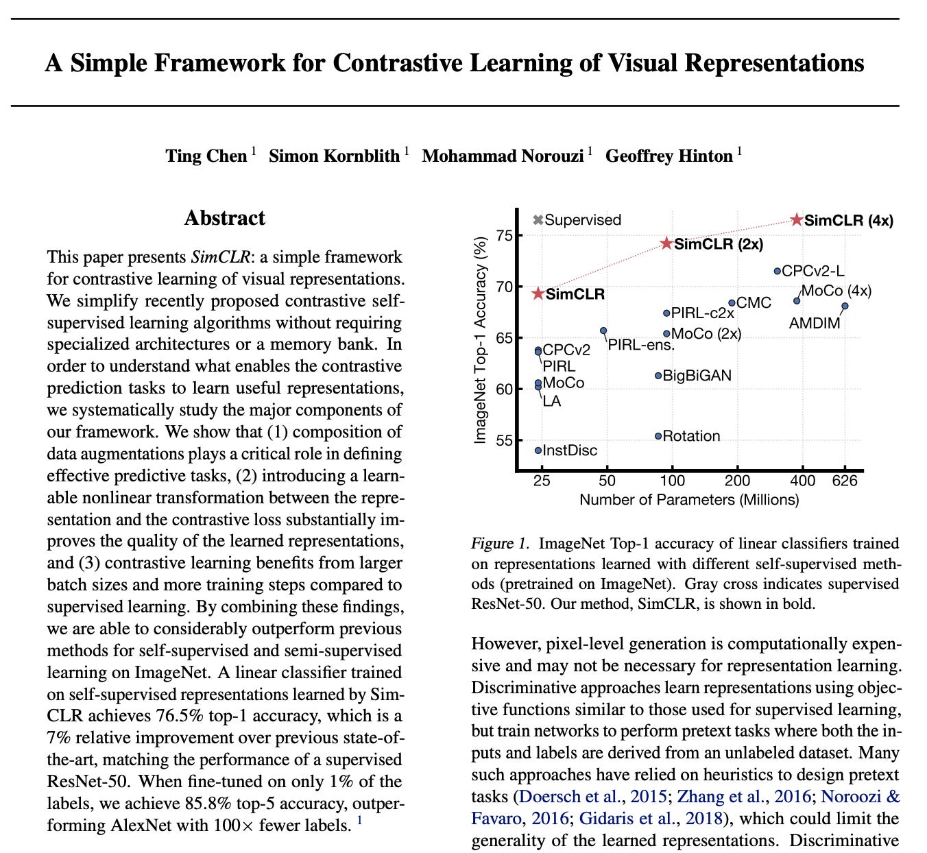
The main goal of contrastive learning is to bring similar pairs (called positive pairs) closer together in the embedding space, and to push dissimilar pairs (called negative pairs) farther apart. This idea was introduced in a 2020 paper titled “A Simple Framework for Contrastive Learning of Visual Representations” published on arXiv. At this time of this writing, the paper has 28600+ citations, which is huge.

The paper that introduced contrastive learning in 2020.

In simple terms the idea of contrastive learning is this:

If two images show the same object (say, a dog from two angles), they should have similar embeddings.

If two images show different objects (say, a dog and a car), their embeddings should be far apart.

In this image, all the examples are positive pairs.

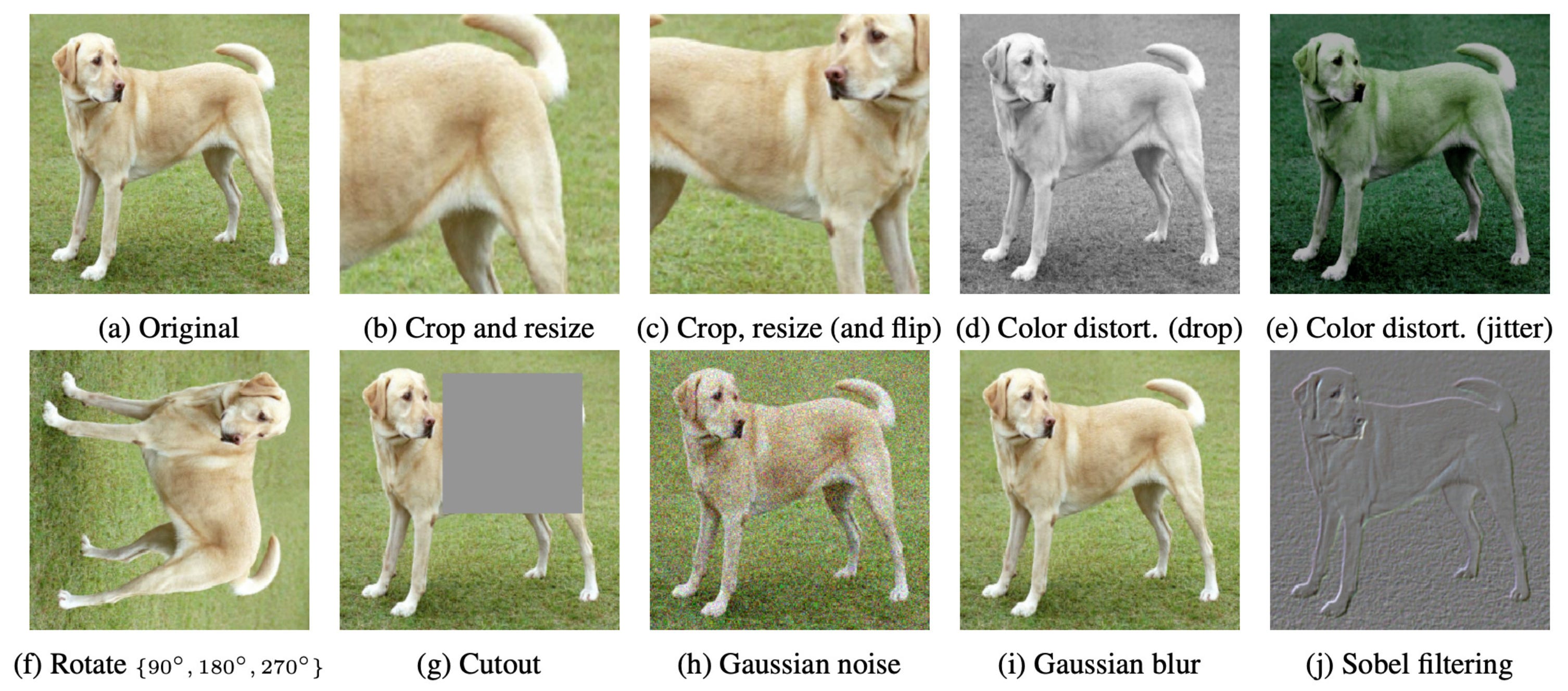
Positive pairs: Represent the same underlying concept (for example, an image and its augmented version, or an image and its correct caption).

Negative pairs: Represent different concepts (for example, two unrelated images or mismatched image-text pairs).

The goal is to minimize the distance between anchor and positive example and maximize the distance between anchor and negative example. Anchor is simply the original image under consideration against which you are comparing other images in the dataset.

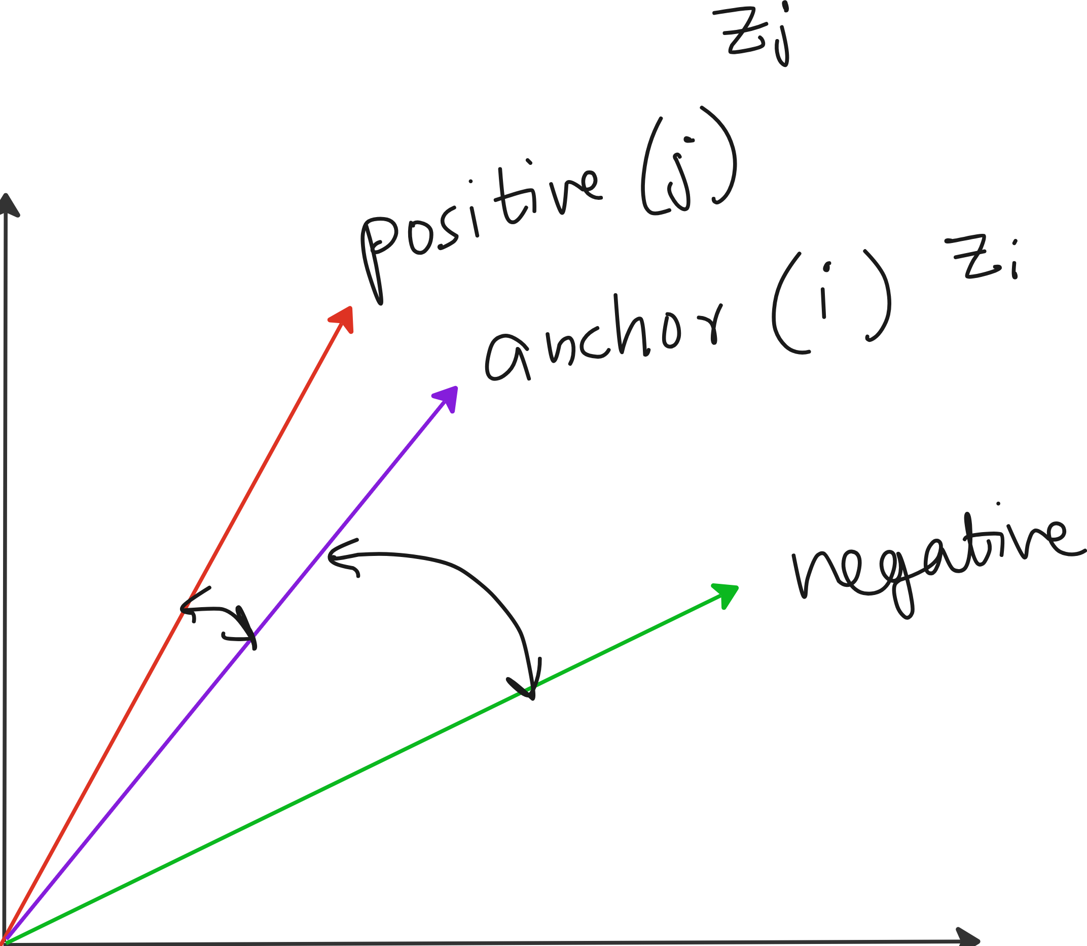
Below is another figure that nicely illustrates the concept of anchor, positive pair and negative pair.

Anchor has high similarity with positive example. Which means the embeddings corresponding to those should have good similarity. Alternately, the distance between those pairs should be less. The top 2 images are positive pairs. The bottom 2 images are negative pairs. Their distance function should be maximized or the similarity should be minimized.

Contrastive loss formula

Let us consider the example of positive pairs to understand the contrastive loss formula. This is used in the famous CLIP paper from OpenAI: https://arxiv.org/abs/2103.00020

I am pasting my hand-written explanation of my formula here. So please excuse the lack if beauty of my hand-writing.

Say these are the vector representations of 2 positive pairs we are considering. We want to maximize the similarity between them.

What is an easy measure of similarity? Cosine similarity. So we can try to maximize cosine similarity. Remember: Cosine similarity is also the same as the dot product between 2 normalized vectors as shown below.

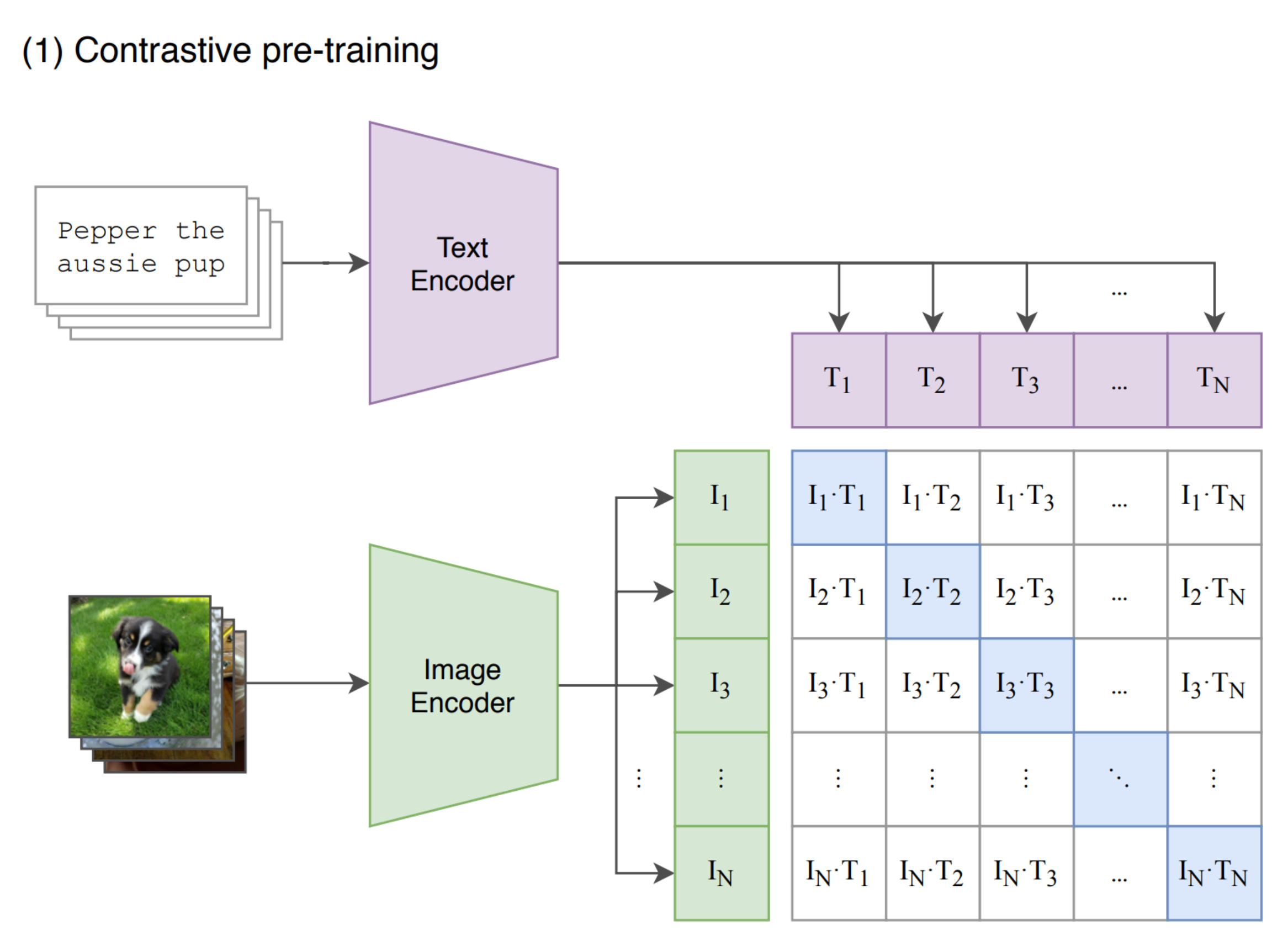
Now we have multiple pairs in our dataset. Consider that the pairs are images and corresponding captions. Because if you have a VLM, you will have embeddings of text and images from an image-caption dataset. If you have N text and image embeddings, you can construct N*N pairs and calculate the cosine similarity.

Your goal is to make sure that pairs that are actual image-caption pairs should have high similarity.

So where can we start?

Firstly it will be great to have a probability distribution of similarity scores. How to convert bunch of numbers to probability scores? Take softmax.

We can introduce an additional parameter to change softmax sensitivity. This parameter will be 𝜏. This is a standard practice.

Now these are similarity scores that lie between 0 and 1. We want to convert this to loss. When similarity is high, loss should be low and vice-versa. How to do that? Take -log() just like cross-entropy loss.

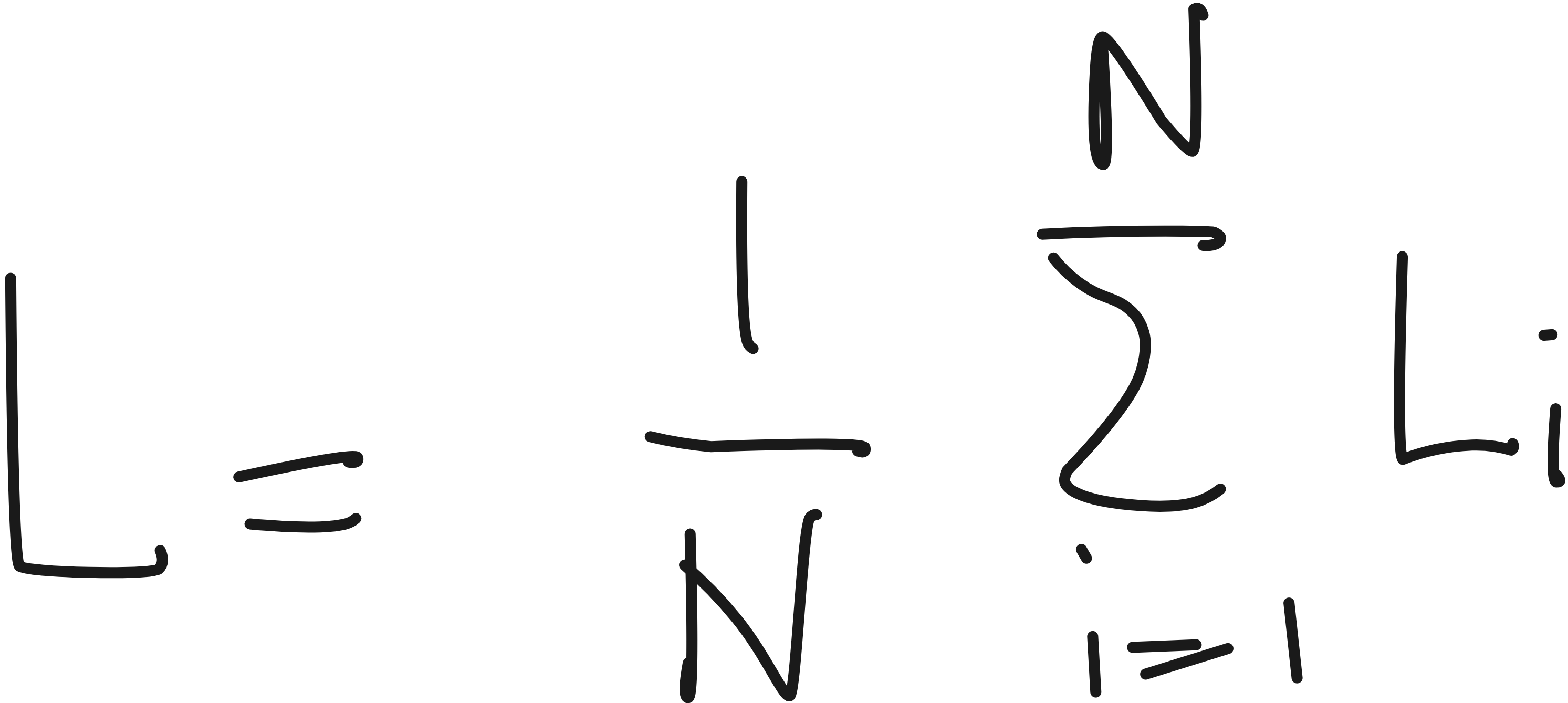
Here “i” is the anchor point and “j” are the other points we compare i against.

Now i can be any point in the N examples. Because any point can be considered as an anchor to compare against the available pairs.

Thus, the total contrastive loss is average over all anchors in the batch.

So, the negatives are implicitly present in the denominator, competing against the positive pair. The loss becomes low only when:

• The similarity between positive pair is high, and

• The similarity between negative pairs is low

Contrastive Language-Image Pre-training (CLIP)

Now that we understand contrastive loss, let us discuss CLIP paper a bit because that is one of the most famous VLMs.

CLIP draws inspiration from contrastive learning.

Here you have N image-caption pairs. They are converted to vectors. Ti is a text vector and Ii is an image vector. Now you need to maximize similarity between Ti - Ii and minimize similarity between Ti - Ij.

Classification problem can be handled using a pre-trained VLM by converting the classes to caption using additional prompt.

This is the final contrastive loss formula. Looks ugly and intimidating when you don’t know what is going on. But this is actually simple.

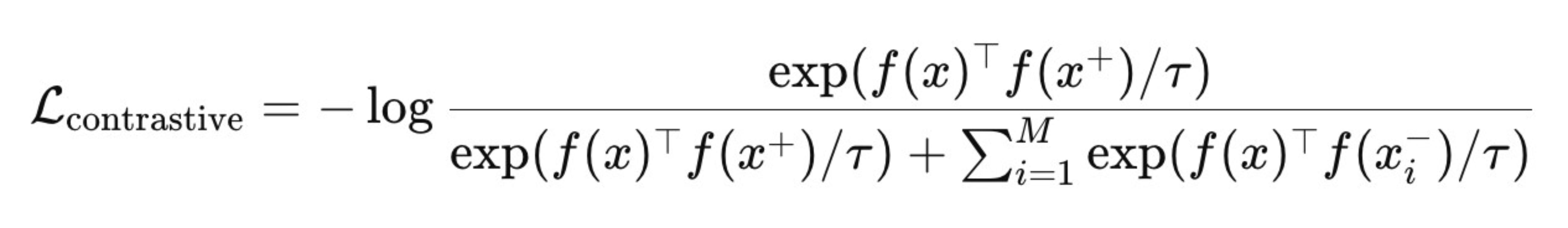
Each image x (called the anchor) is paired with:

• One positive example x+: usually an augmented version of the same image (for example, a rotated or cropped view of the same polar bear).

• Several negative examples xi−​: other images from the batch (for example, the lemur, bird, or deer shown in the image).

So, for every anchor image, the model has exactly one correct match and many distractors.

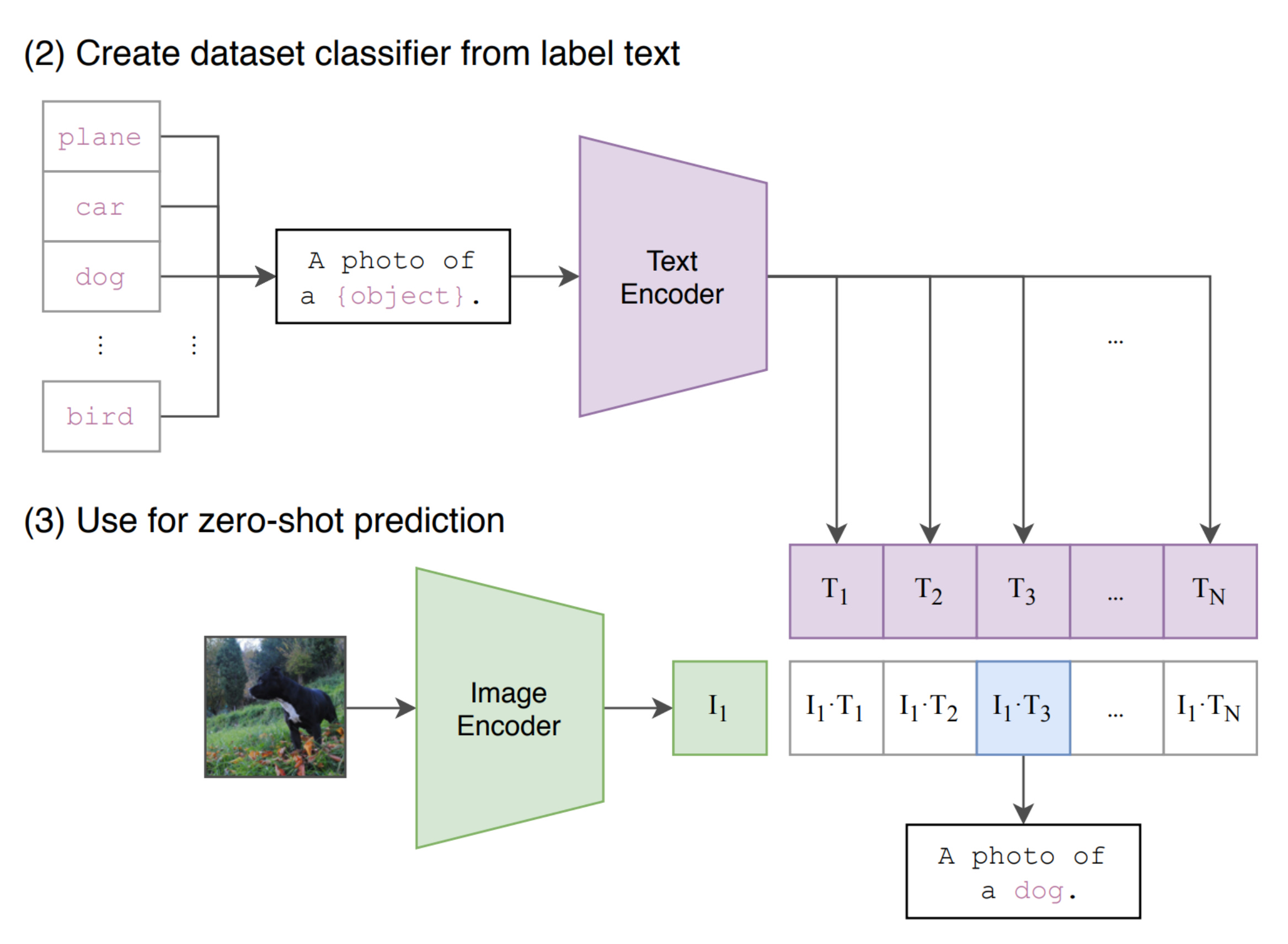
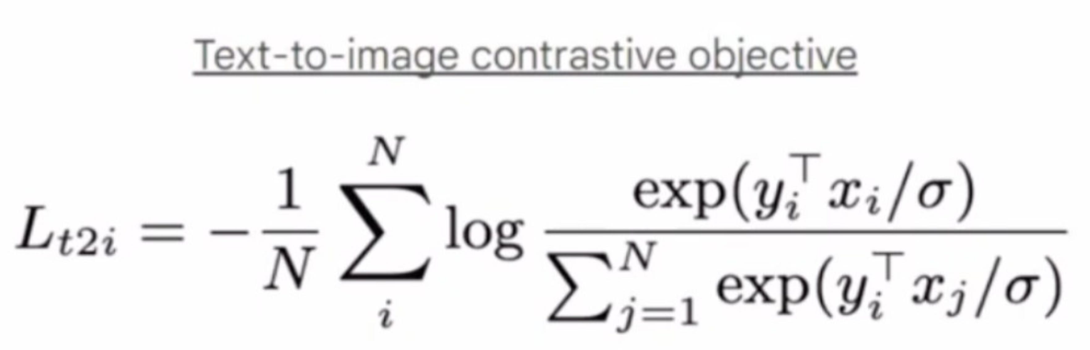
In image-caption pair dataset, we can have 2 objectives.

1. Retrieve image that fits a caption

2. Given an image, provide the best caption

For these 2 objectives we can have 2 different losses. Pretty straightforward equation once you understand the basic idea behind contrastive loss.

Let us build a VLM

Now let us build and train a NanoVLM from scratch. We need to have an idea about the following.

1. Task description

2. Dataset

3. Model architecture

4. Image encoder

5. Text encoder

6. Loss function

Task description

We will build a NanoVLM: tiny CLIP-style model trained on synthetic colored-shape captions. Why “nano”? because number of trainable parameters will be less than 5 million.

Task: For a give text caption, we have to retrieve the best images from the dataset

Dataset

For a given text caption, we have to retrieve the best images from the dataset. We will use a synthetic small dataset.

Images are shapes with different colors and positions. Captions literally mention the color, shape and position in one string.

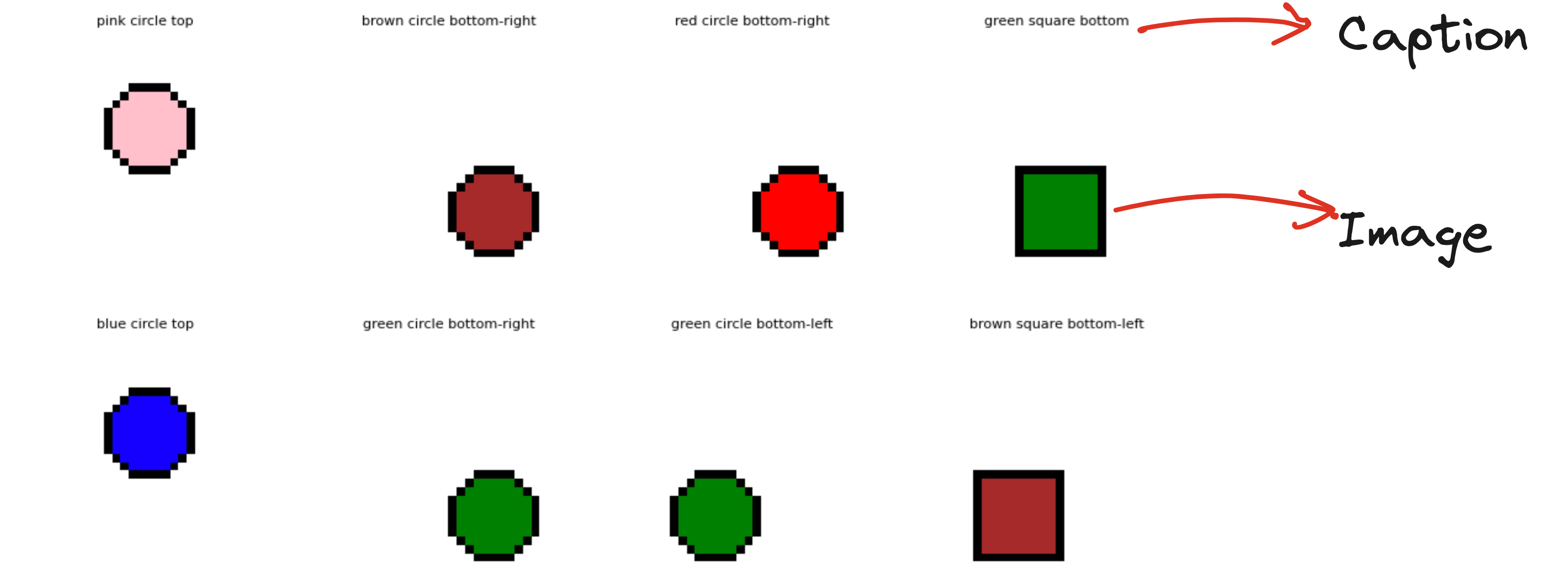
It is easy to create this synthetic dataset if we use parameters like below.

Overall model architecture

This is a tiny CLIP-style Vision-Language Model (VLM).

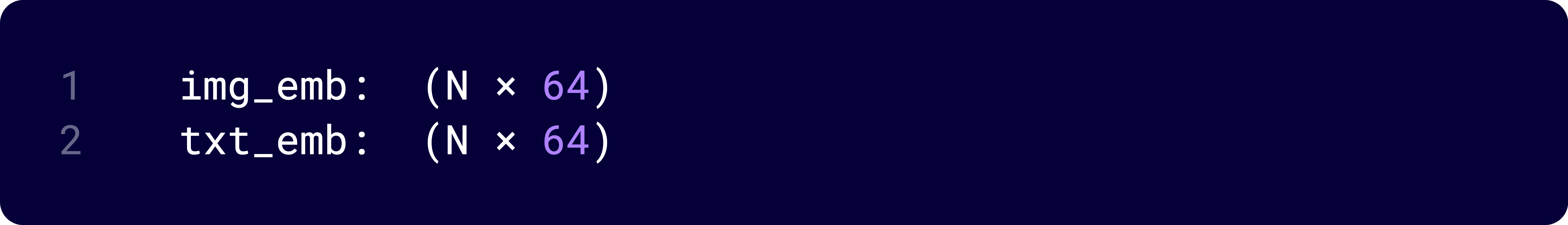
It has two separate encoders - one for images and one for text.

Both encoders map their inputs into a common embedding space of dimension 64 (or other dimension we choose).

The goal is to make matching image-text pairs lie close together in this space.

This is the simple architecture of VLM we are going to build

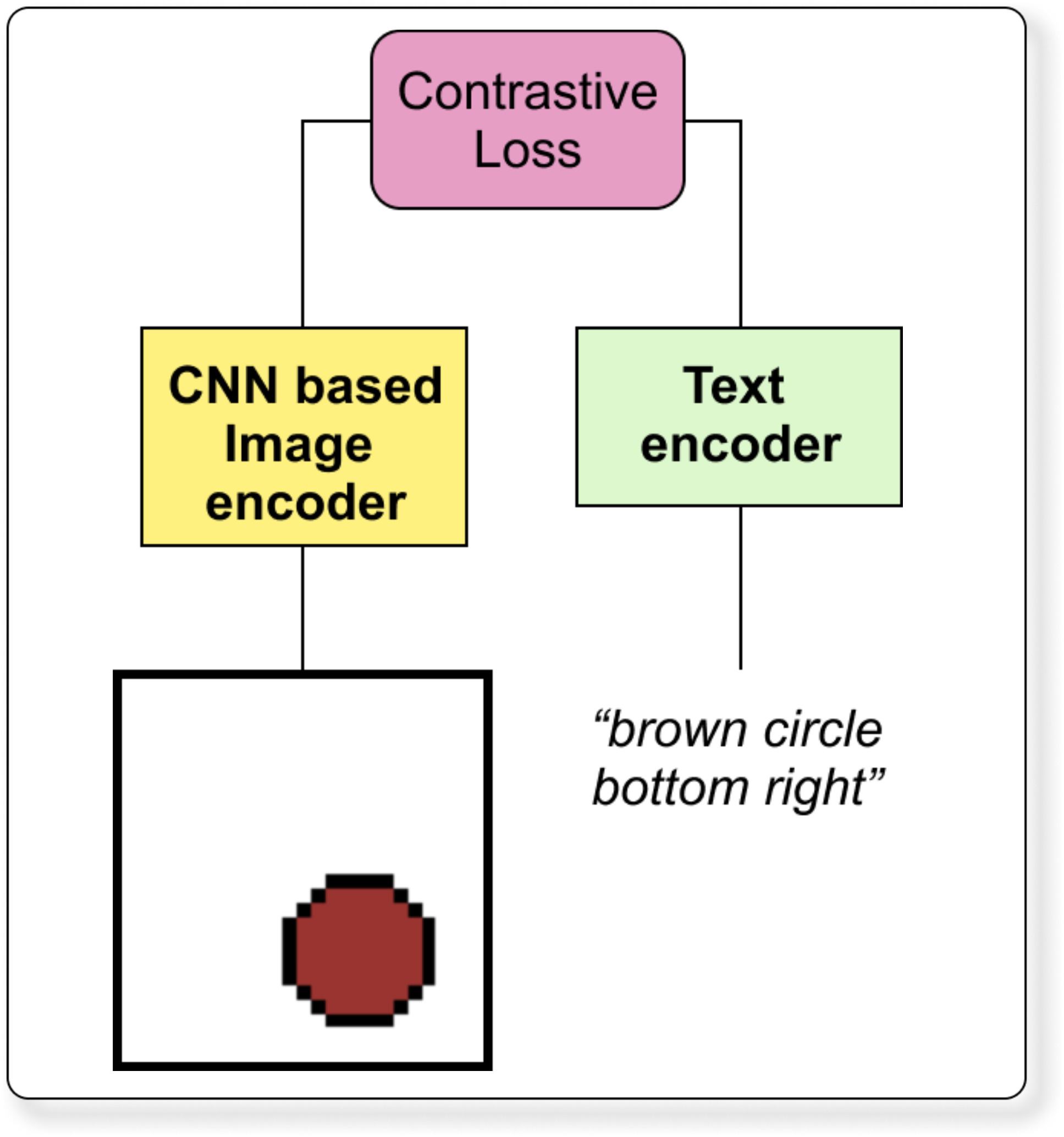
Image Encoder

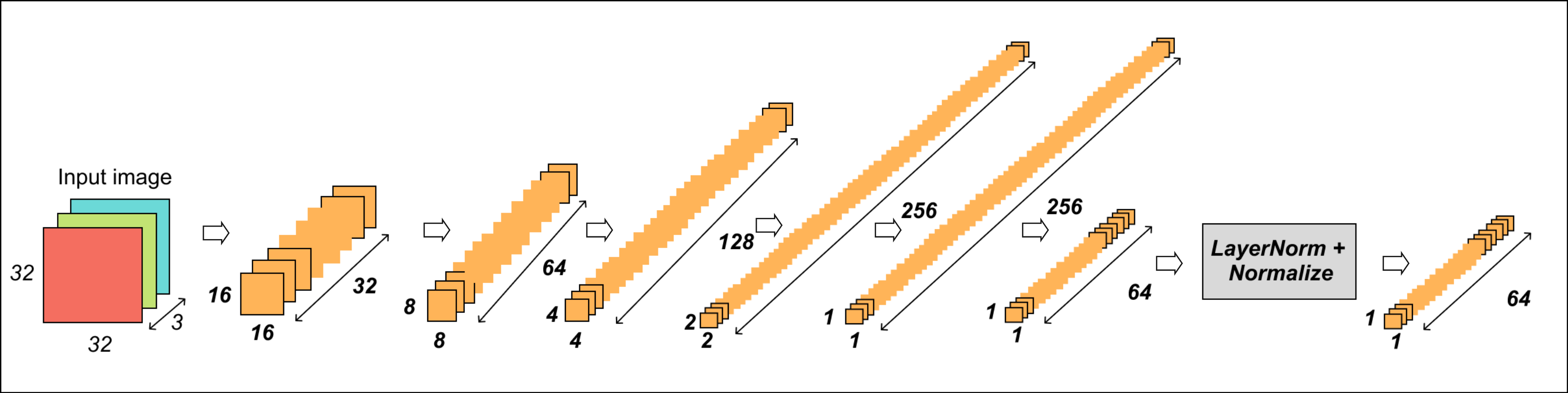
• A small CNN (4 convolutional layers) progressively downsamples the input image.

• After the convolution blocks, a global average pooling layer reduces spatial features.

• A linear projection maps to the embedding dimension.

• Finally, a LayerNorm + L2 normalization ensures embeddings are unit vectors (important for cosine similarity).

The CNN architecture is shown below.

The architecture of the image encoder we are using in this VLM

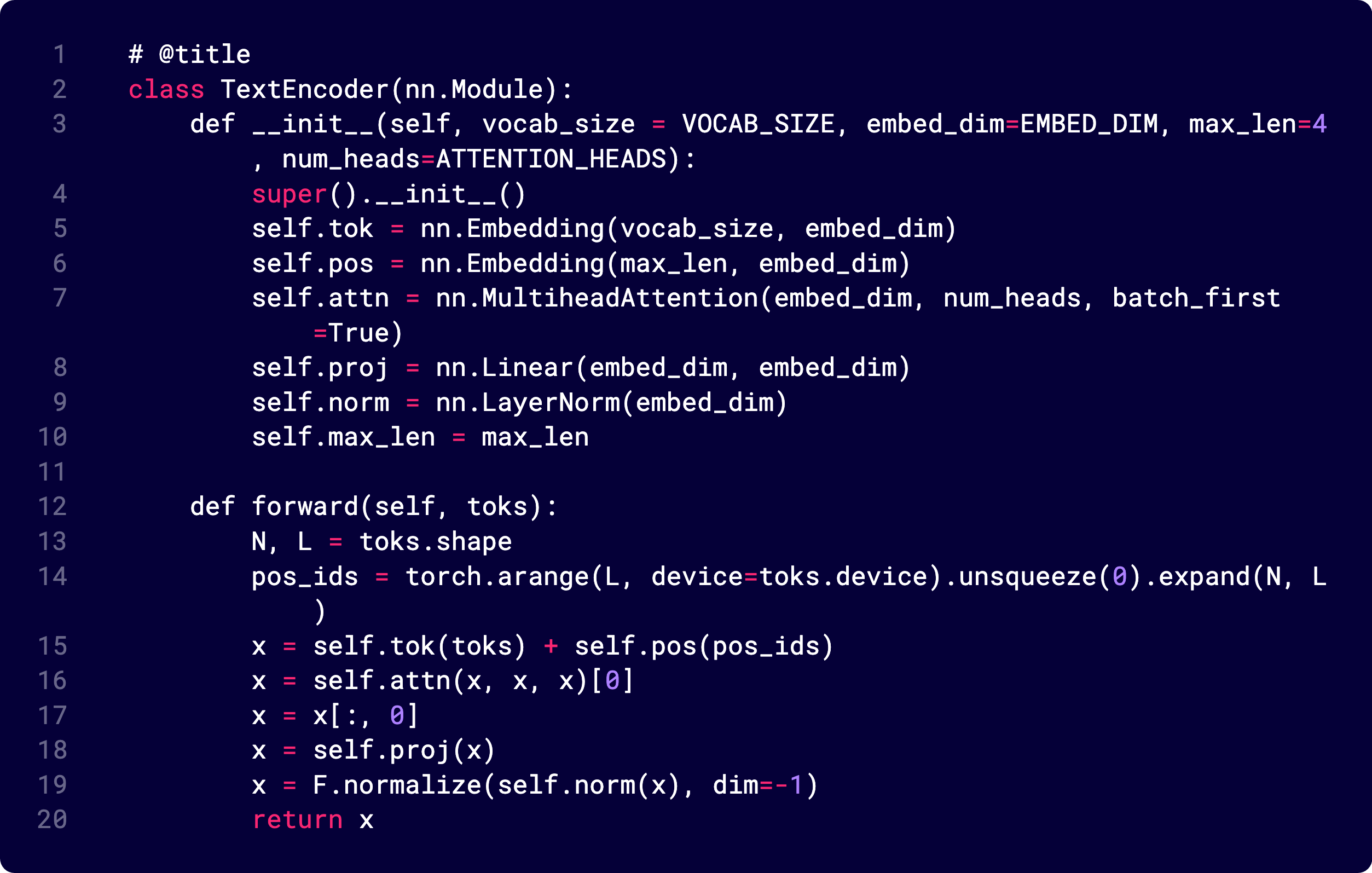
Text Encoder

• Each caption has tokens like [CLS] red triangle left.

• A token embedding layer converts each word to a 64-d vector.

• A positional embedding layer adds position info (like transformers).

• MHA after this

• Followed by a Linear layer + LayerNorm + L2 normalization.

The code below shows a layer-by-layer breakdown of the text encoder.

Loss function

The loss attempts to align the image and text embeddings such that:

• Matching pairs (correct caption for image) have high similarity.

• Non-matching pairs have low similarity.

Compute embeddings for a batch:

Compute similarity matrix:

Each row i compares image i with all text embeddings.

Diagonal elements are the correct image-text pairs.

Apply Cross-Entropy Loss in both directions

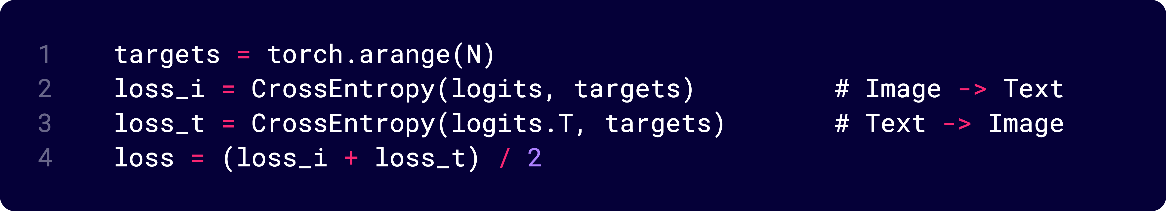
Image ➝ Text classification

Text ➝ Image classification

This is symmetric contrastive learning, exactly like CLIP.

I am not pasting the full code here, but I will show you how the embeddings look before and after training.

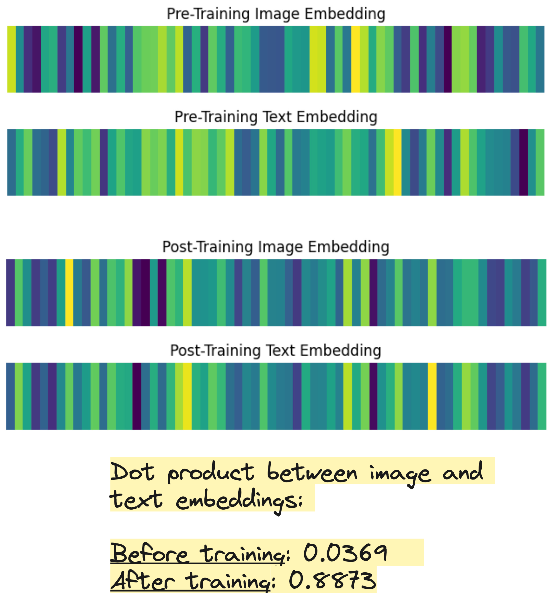
Embedding similarity before and after training

Look at the beautiful color bands below. Each color shows the value of the embedding vector along a particular dimension. Totally there are 64 dimensions. Look at how similar the embeddings look after training. So beautiful.

I also tried 3D embeddings instead of 64-D embeddings so that visualization can be exactly like vector embeddings. Here are the results.

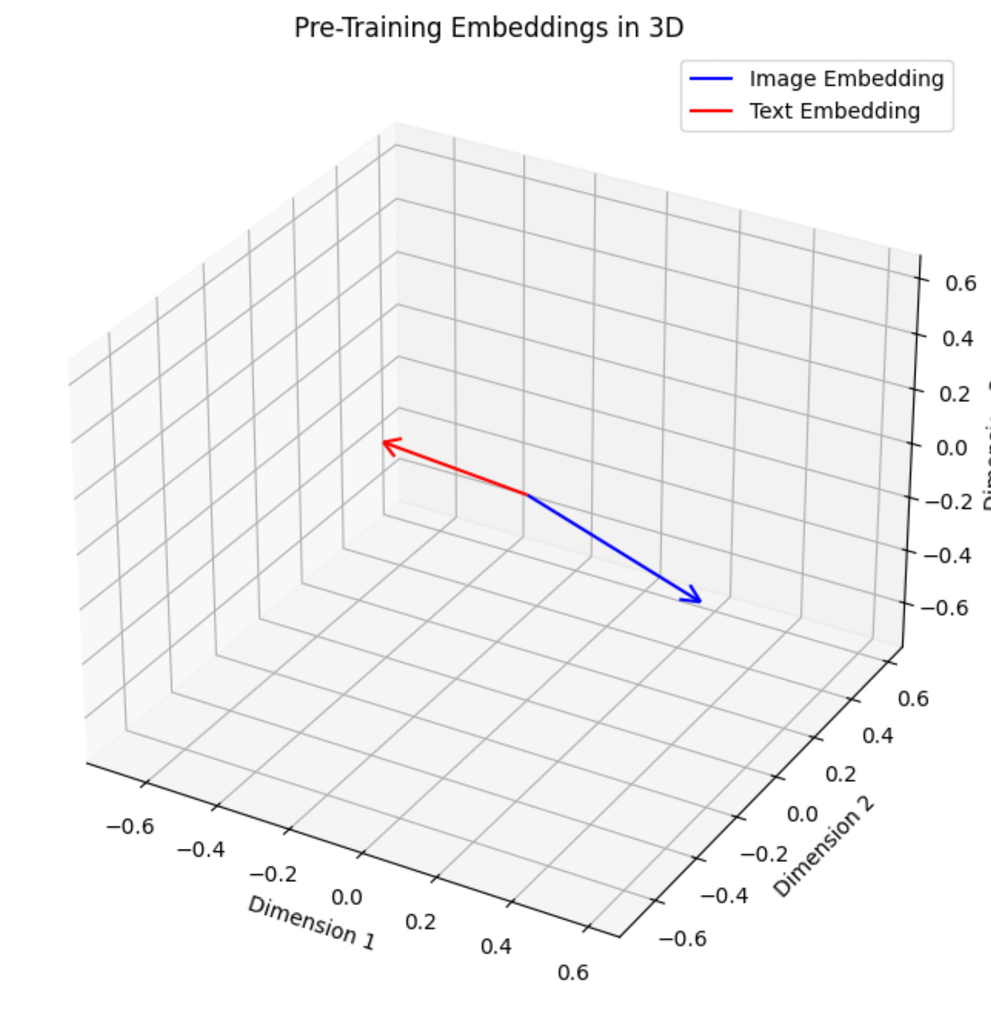
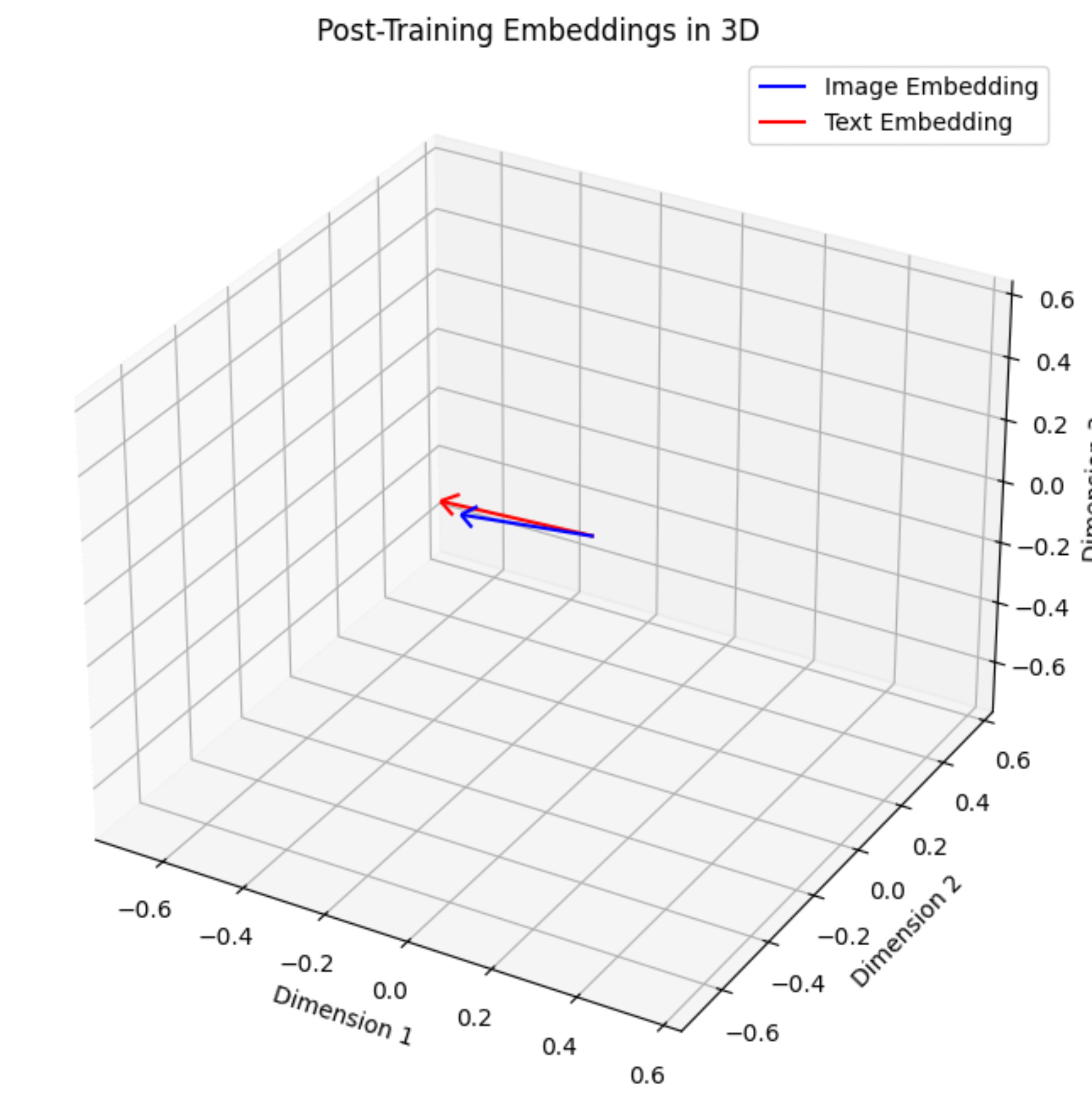
I think this is a great example to show how the image and text embeddings align after training in a VLM.

Why is this model called “Nano”?

We can answer this question by simply hand calculating the total number of trainable parameters.

We can calculate the trainable parameters separately for text encoder and image encoder.

Image Encoder: Number of parameters

Image encoder is a CNN with a total of around 440k trainable parameters. I am not going to show you the entire math of how for each layer I have calculated these parameters but I will show you the layer-wise distribution of the parameters.

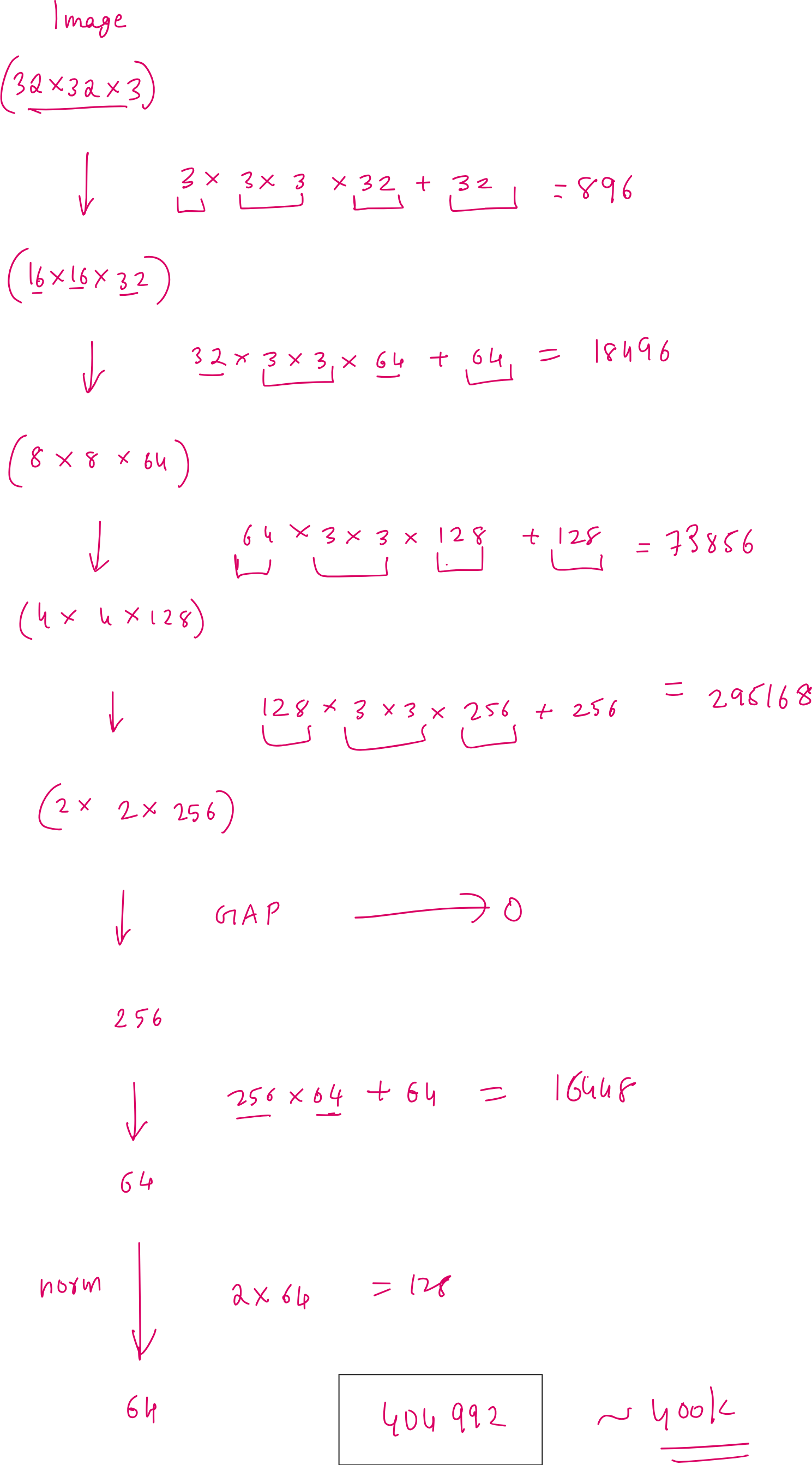
Just notice that the early layers of a CNN does not contribute to that many number of trainable parameters. The more convolutional layers you add later, the more your number of trainable parameters increase at a faster rate. So if you care about making your image encoder lightweight, you should reduce the number of layers that come later. The logical reason why this happens is because later layers have more number of channels that are produced at the output of convolution operation and for every channel you need a separate filter. Thus total number of filters in a given layer is same as the total number of channels that their layer produces at the output.

I simply encourage you to perform this calculation yourself if you don’t know how to calculate the number of parameters in a given convolution layer I am linking a video here this will definitely help you. This is a short ~20 minute video that I recorded recently to explain what exactly does filters do dimensionality wise in a convolution operation:

Now let us also calculate the total number of trainable parameters in the text encoder.

Text Encoder

Like the Image Encoder, I am not going to show the entire calculation, but I’ll show the layer-wise distribution of parameters.

Pardon my atrocious hand-writing once again.

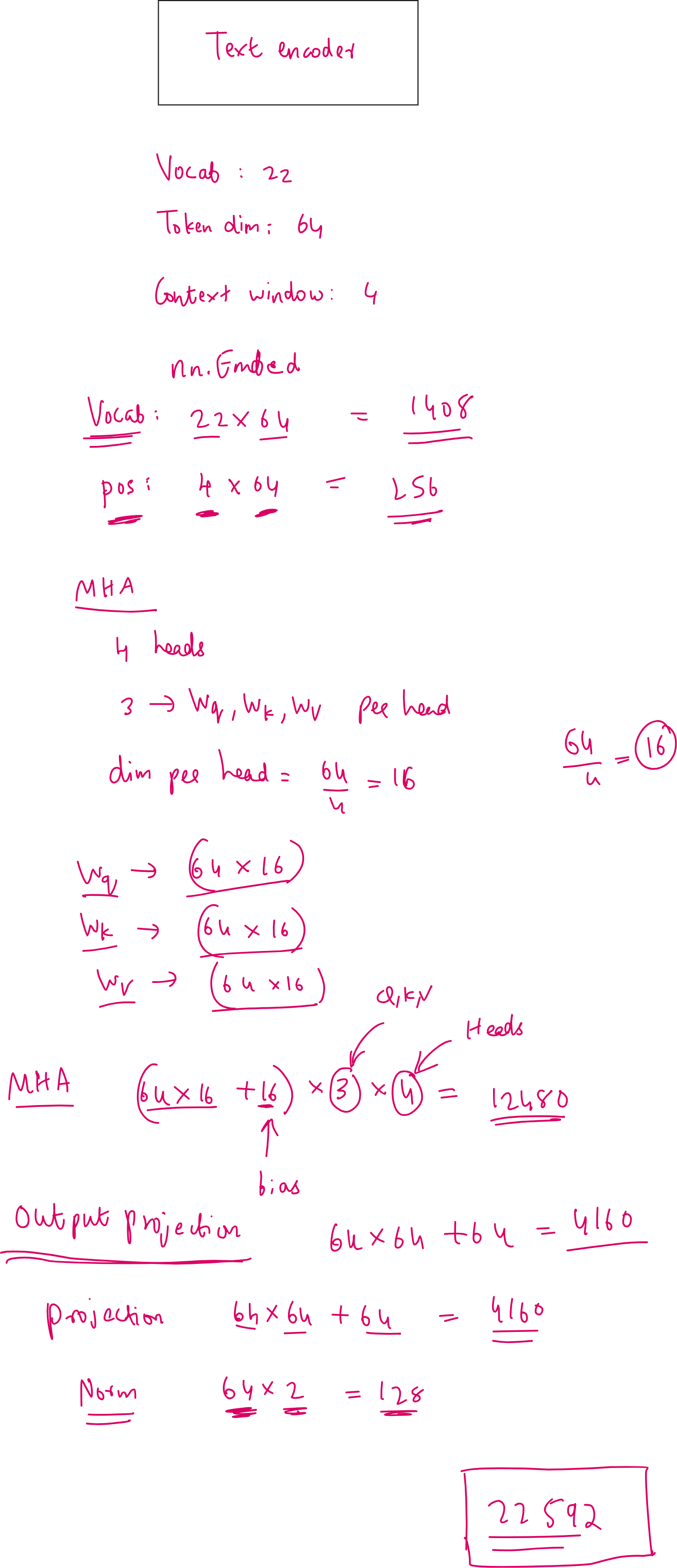
The total number of parameters contributed by the text encoder is just 22.5k. This is only 5% as that of the image encoder. The total number of parameters is less than 500k. And this is the reason why we are calling this as a “nano” vision language model.

Conclusion

This exercise of building NanoVLM from scratch was done as part of a series called “Transformers for Vision.” If you wish to watch the full lecture video, you can have a look at it here. You can code along with me in the video to learn how to build this Nano VLM completely from scratch yourself:

If you wish to get access to our code files, handwritten notes, all lecture videos, Discord channel, and other PDF handbooks that we have compiled along with a code certificate at the end of the program, you can consider being part of the pro version of the “Transformers for Vision Bootcamp”. you will find the details here:

https://vision-transformer.vizuara.ai/

Other resources

If you like this content, please check out our research bootcamps on the following topics:

CV: https://cvresearchbootcamp.vizuara.ai/

GenAI: https://flyvidesh.online/gen-ai-professional-bootcamp

RL: https://rlresearcherbootcamp.vizuara.ai/

SciML: https://flyvidesh.online/ml-bootcamp

ML-DL: https://flyvidesh.online/ml-dl-bootcamp