
Vision Transformers
Understanding and fine-tuning Vision Transformers (ViT) for image classification, to hands-on transfer learning with pretrained models.

Table of Contents
Adapting transformers to images: patch embeddings and flattening
Positional encodings in vision
Encoder-only structure for classification
Benefits and drawbacks of ViT
Real-world applications of ViT
Hands-on: fine-tuning ViT for image classification
Finetuning Vision Transformer Code is available below
https://github.com/VizuaraAI/Transformers-for-vision-BOOK
1.1 Introduction to Vision Transformers and Comparison with CNNs
Vision Transformers adapt the transformer architecture from language modeling to images. Instead of scanning an image with small sliding filters, they treat small image patches as tokens and learn how these patches relate to one another through self attention. For now it is enough to think of a Vision Transformer as a model that can look at all parts of an image at once and decide which regions should influence each other.
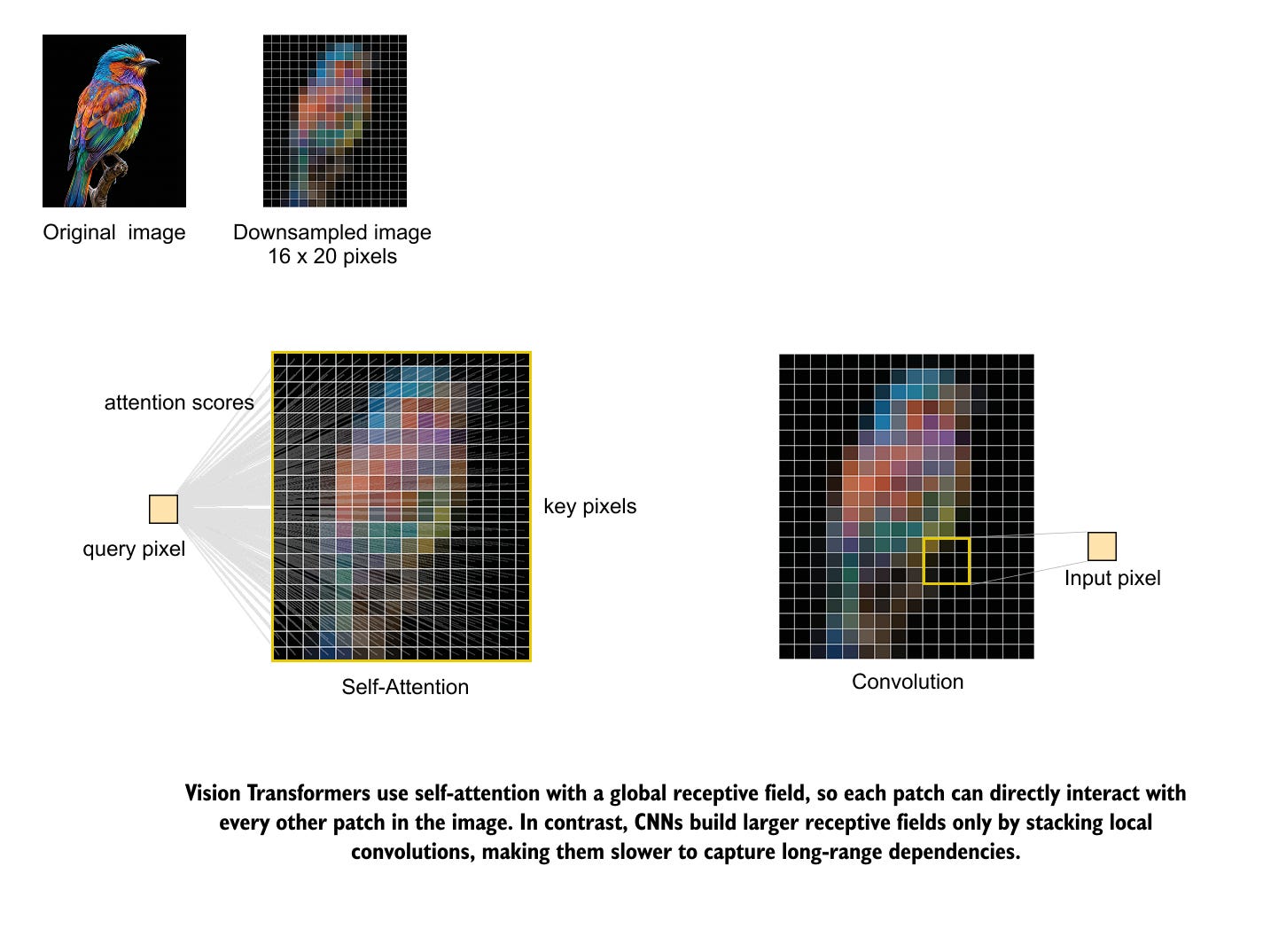
The key architectural difference between Vision Transformers and convolutional networks lies in how they see an image. A convolutional layer only looks at a small neighborhood of pixels when it computes its output. Its receptive field grows only gradually as we stack more layers and pooling operations. This locality bias has been very successful for classic vision tasks, but it means that long distance relationships in an image are only captured indirectly and late in the network. Figure 1 illustrates this contrast between global self attention and local convolution on a simple bird image.
Self attention in a Vision Transformer has a global receptive field from the first layer. For any query location, the model can compare it directly with every other patch in the image and decide which ones are relevant. In the bird illustration, a single pixel or patch can immediately connect to any other region in the picture, while a convolution sees only its nearby neighborhood and must rely on many stacked layers to move information from one side of the image to the other.
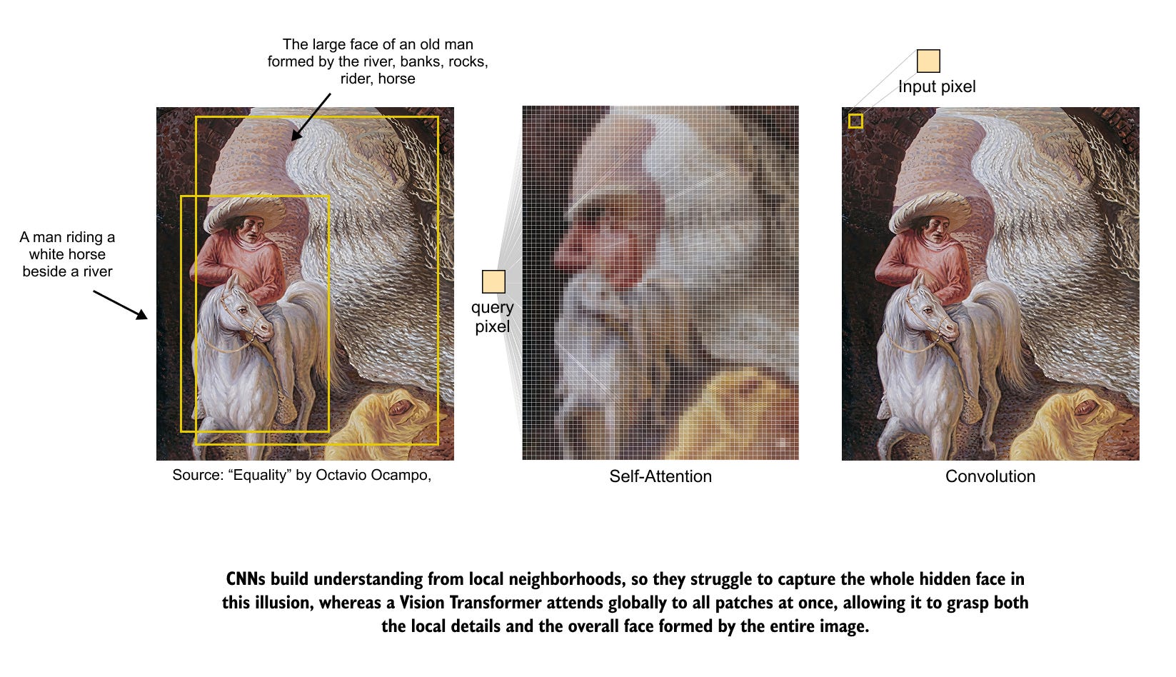
The second figure we have an optical illusion painting to make this difference more concrete. A human viewer can perceive both the detailed scene of a rider by the river and the larger face formed by the entire painting. A convolutional model tends to focus on the local textures of rocks, water, and fur, while a Vision Transformer can link distant regions that together form the face. Figure 2 shows how self attention attends across the whole painting, while a convolution still operates on a restricted local view.
The classic story of several blind people trying to describe an elephant gives another intuitive picture of this difference. Each person touches a single part and concludes that the elephant is a rope, a wall, or a snake, depending on whether they hold the tail, the body, or the trunk. A convolutional network behaves in a similar way, since each unit only has access to a small patch and builds its understanding from many separate local views. A Vision Transformer behaves more like a group that can share information freely. Even if each observer starts with a limited view, self attention lets them combine their observations and agree on the full shape of the elephant.
In the rest of this chapter we shift from this high level comparison to the inner workings of Vision Transformers. We will unpack how images are converted into patch tokens, how positional information is added, and how self attention layers process these tokens. Step by step, we will build up the full Vision Transformer encoder and its classification head so that the complete architecture becomes clear and concrete.
Since we've already covered the fundamentals of Transformers, I won't be going into too much detail here. If you're new to the architecture, I highly recommend reading my previous post, to get a solid foundation before we dive into Vision Transformers.
From Text Transformers to Vision Transformers
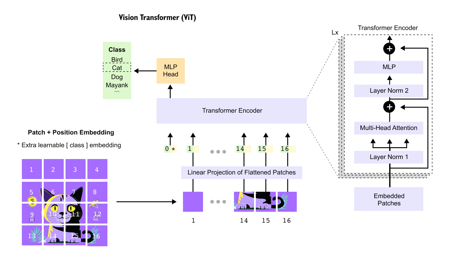
Transformers for text and transformers for images share the same core ideas. In language models such as GPT, we start from a sequence of tokens, embed them, and apply masked self attention so that each token can only attend to tokens at its current or earlier positions. This matches the next token prediction objective, where the final context vector of the sequence is used to predict the following token. In Vision Transformers, an image is first tokenized into a sequence of patches, self attention is applied without masking so that every patch can attend to every other patch, and a special class token provides a single representation that is passed to a small MLP head for classification.
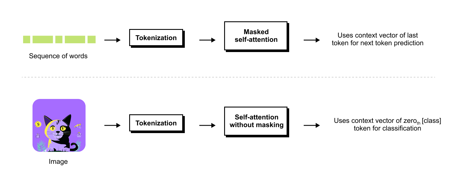
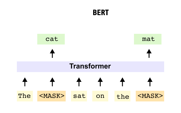
BERT provides a second reference point for Vision Transformers. Instead of predicting the next word, BERT is trained to recover masked tokens inside a sentence, so it uses unmasked self attention over the entire sequence to capture bidirectional context. Vision Transformers adopt this encoder style design from BERT, but apply it to image patches together with a class token, giving a close analogue of BERT style sequence understanding in the image domain.
Now that we have compared transformers for text and images at a high level, we can focus on how a Vision Transformer actually sees an image. In the next section we will follow an image as it is cut into small patches, converted into vectors, and arranged into a sequence that looks very much like a sentence of tokens. This patch embedding stage is the first step that lets a standard transformer encoder operate directly on images.
1.2 Adapting transformers to images: patch embeddings and flattening
Adapting a transformer to images starts with a simple question: how can we turn a 2D image into the kind of 1D token sequence that a text transformer expects? Vision Transformers answer this by cutting the image into a grid of fixed size patches and treating each patch as a token. In this section we work through that patch embedding step using the 640 by 640 cat image and then show two common implementations: a flatten plus linear projection and an equivalent convolutional layer.
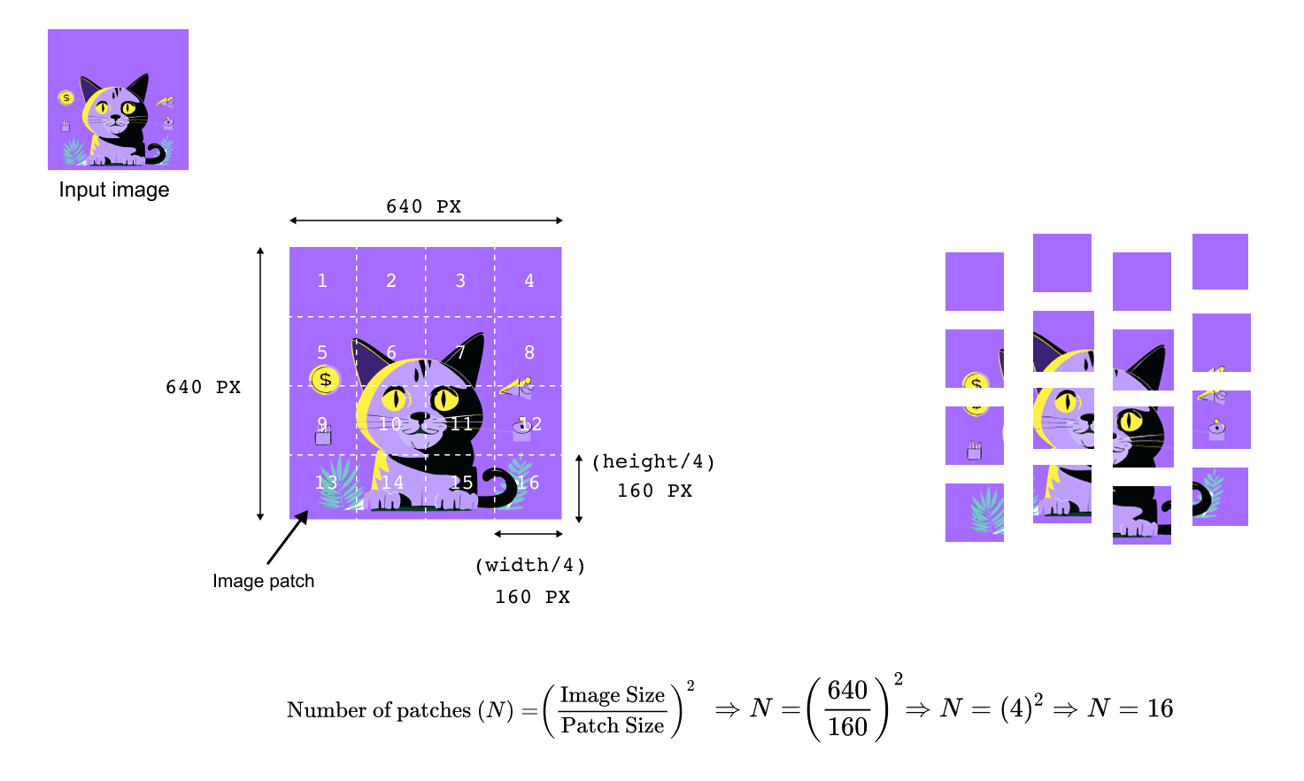
For the cat example, suppose the image has height and width 640 pixels and three color channels. We choose square patches of size 160 pixels. The image is divided into a 4 by 4 grid of non overlapping patches, each 160 by 160 by 3. In general, for an image of height H, width W, and patch size P, the number of patches N is
assuming H and W are multiples of P. For a square image of side S this reduces to
With H = W = 640 and P = 160 we obtain N = (640 / 160)² = 4² = 16 patches.
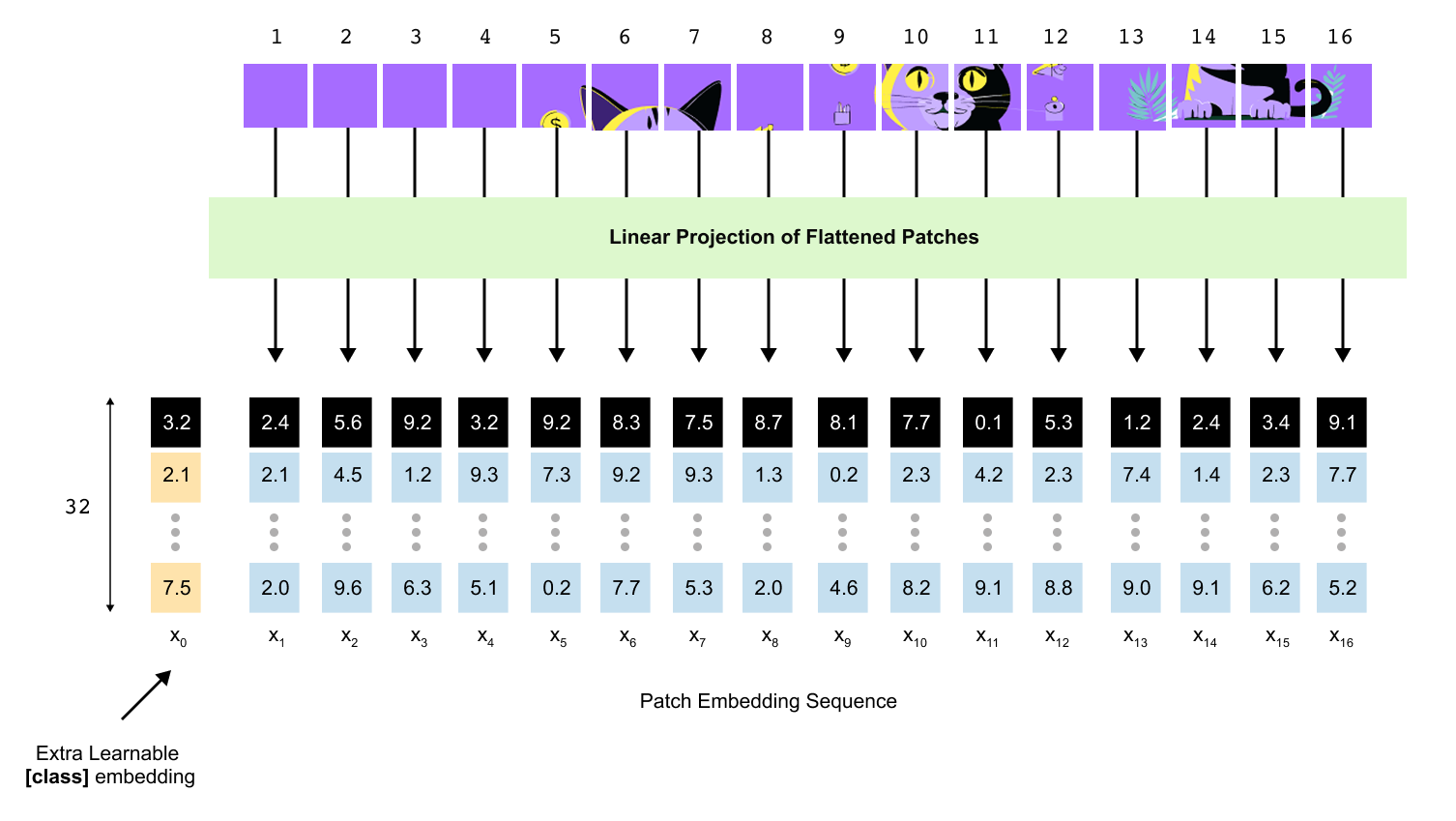
Once the image has been split into patches, each patch must be converted into a vector that lives in a common embedding space of dimension D, just as word tokens are embedded in text models. One straightforward approach, used in the original Vision Transformer paper, is to flatten each patch and apply a linear projection. A single patch has shape P by P by C, where C is the number of channels. Flattening gives a vector of length P²C.
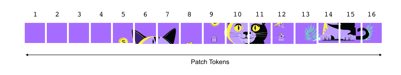
In the transformer it is convenient to line these patches up in a fixed order and think of them as a one-dimensional sequence rather than a two-dimensional grid. For instance, we might start from the top-left patch, then move left to right, row by row, until we reach the bottom-right patch.
Patch embeddings without convolution
In the first subsection we will build patch embeddings without any convolutional layers. We will treat each 160×160×3 patch as a tiny image, flatten all of its pixels into a long vector, and pass that vector through a learnable linear layer to obtain a D-dimensional patch embedding. This view mirrors word embeddings in language models: each patch is simply another token whose embedding is learned directly from data.
To keep things concrete, return to the 640×640 cat image from the previous section. We divide it into a 4×4 grid of non-overlapping patches, each of size 160×160 pixels.
Each of these sixteen patches will become one token for the transformer.
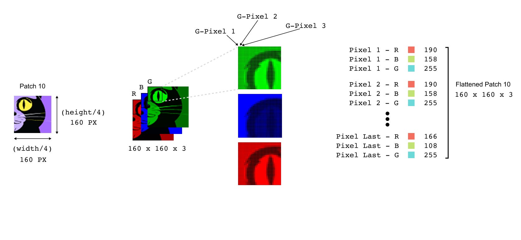
Consider patch 10, the square around the cat’s eye. As an RGB patch it is a small 3-D tensor with shape
where C=3 is the number of colour channels. The image in Figure 7 shows this patch split into its red, green, and blue planes, and then shows a few individual pixels as (R,G,B) triplets. The first step of the non-convolutional patch embedding is to flatten this tensor into a single vector by concatenating all pixel values from all channels in a fixed order. If we denote the flattened version of the i-th patch by flat_patch_i then its length is
For a 160×160 RGB patch this means
numbers per patch. Flattening does not learn anything; it is just a reshaping operation that turns a 160×160×3 block of pixels into a vector of length 76,800.
A transformer, however, does not want raw pixel vectors of length 76,800. It expects a much shorter embedding vector of some dimension D, such as D=32 in our toy diagrams or D=768 in a ViT-Base model. The simplest way to obtain that is to apply a shared linear layer to every flattened patch. We introduce a weight matrix W_patch and a bias vector b_patch and define the patch embedding for the i-th patch as
with
The dimensions line up in the natural way: W_patch takes a length-P^2C vector and maps it down to a length-D vector, while b_patch shifts the result. In the cat example, if we choose D=32, then W_patch has shape 32×76,800 and b_patch has length 32. The output
is a D-dimensional patch embedding. The same parameters W_patch and b_patch are reused for every patch in every image, so they are heavily shared and trained end-to-end with the rest of the model. You can think of each row of W_patch as a learned template that looks at the entire patch and responds with a single number; stacking D such responses gives the embedding vector.
At this point we have turned one patch into one token. Repeating the same flatten-and-project operation for all N patches yields a collection of patch embeddings
We arrange them in a fixed, deterministic order, for example row by row across the image, and stack them into a matrix
This matrix is the direct analogue of the token-embedding matrix in a text transformer. The only difference is that each row now encodes an entire 160×160 coloured region of the image instead of a word or subword.
It is helpful to interpret this as describing the whole pipeline. Before embedding, the model sees N raw patches, each of shape 3×P×P. After flattening we conceptually have N vectors of length 3P^2. After the linear projection we have N patch embeddings of length D. Once we add the special class token and positional embeddings in the following sections, this becomes an (N+1)×D matrix that is finally presented to the transformer encoder.
Patch embeddings with convolution
In this subsection we will see that a single Conv2D layer can perform almost the same job in one shot. By choosing the kernel size and stride to match the patch size, a convolution turns the 640×640 image into a 4×4 grid of feature maps whose channel dimension is exactly our embedding dimension (for example, 32 channels). Each spatial location in this feature map is then interpreted as one patch token.
The idea is that a convolution with kernel size P and stride P can visit each patch exactly once, compress it, and write the output into a grid of size (H/P,W/P)
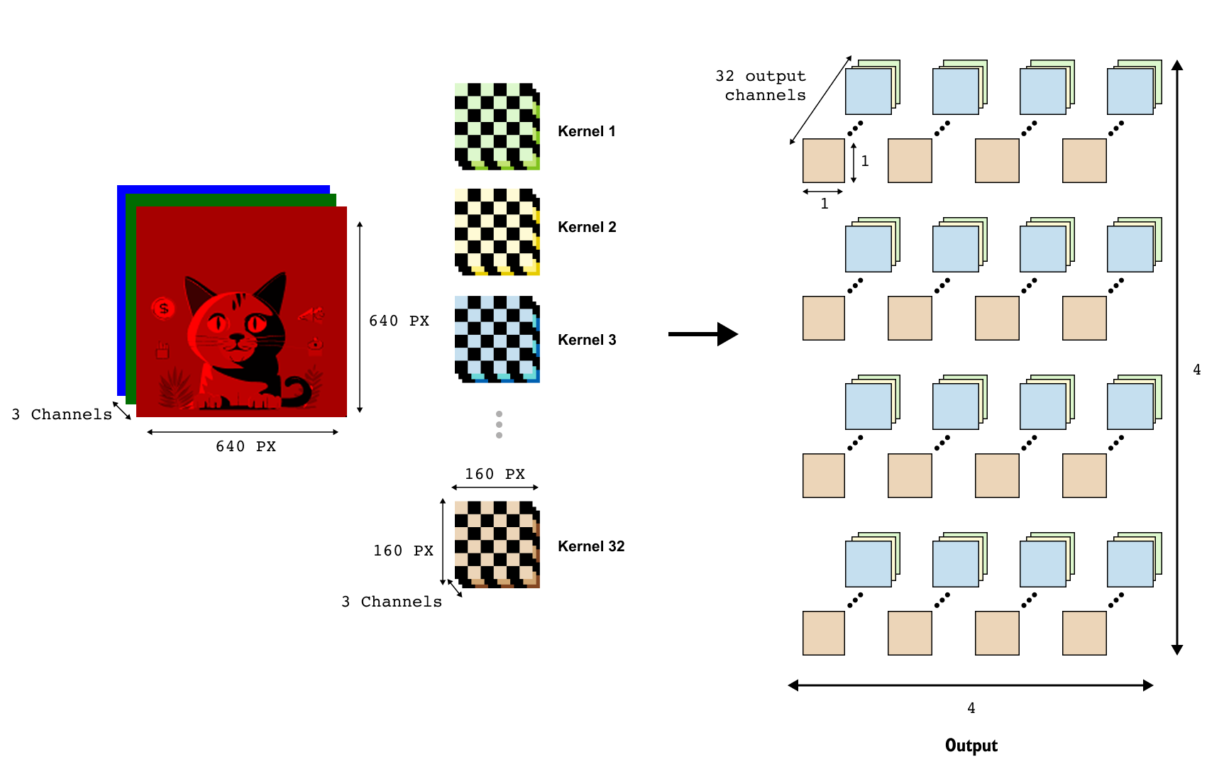
In our running example we use kernels of spatial size 160×160 and stride 160 The input is a tensor of shape (3,640,640). We apply a convolution layer whose RGB image we set C=3. The number of output channels is chosen to be our desired embedding dimension, for example D=32. Both the kernel size and the stride are set to 160, which means the kernel slides over the 640×640 image in non-overlapping 160×160 steps, and we use zero padding so that the image is neatly tiled into patches without any extra border pixels being added.
The convolution layer contains D separate kernels. Each kernel is a learnable weight tensor of shape (C,P,P)=(3,160,160). When the layer processes the image, each kernel slides over the image in steps of 160 pixels, producing one response per patch. Because the stride equals the kernel size, there is no overlap between neighbouring receptive fields. After the convolution, the output tensor has shape
Each spatial location (u,v) in this 4×4 grid corresponds to one patch of the original image. The vector of 32 numbers at that location comes from the 32 kernels, which together play the role of the rows of the linear matrix W_patch in the previous subsection. If we flatten the 4×4 grid of spatial locations into a length-16 sequence, and read out the 32-dimensional vector at each location, we obtain the same set of patch embeddings as before.
Taken together, these two constructions show that Vision Transformers do not depend on any particular patch-extraction trick: what matters is ending up with a sequence of N patch embeddings of dimension D. Whether those embeddings come from flattening plus a linear layer or from a carefully configured convolution is largely an implementation choice; once we have the N×D matrix of patch tokens, the rest of the Vision Transformer proceeds in exactly the same way.
Adding the class token and forming the sequence
So far we have obtained N patch embeddings x1,…,xN, each of dimension D. For classification tasks the Vision Transformer introduces one extra token, called the class token. This token does not come from any particular patch; it is a learned vector that is added to the front of the sequence and is meant to gather information from all other tokens through self-attention.
We denote the class-token embedding by
This vector is a trainable parameter, initialized randomly when we create the model and optimized along with all other weights. Once we have x_0 and the patch embeddings x1,…,x_N, we can form the full sequence matrix.
The number of tokens entering the transformer encoder is therefore
In the 640 by 640 example with patch size 160, this gives N = 16 plus one class token, so there are 17 tokens in total, each of dimension D=32.
that will become the input to the Vision Transformer, once we add positional information.
1.3 Positional encodings in Vision Transformers
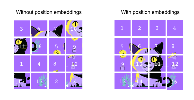
Self-attention in a Vision Transformer has no built-in notion of order. In the left panel of Figure 10, we could shuffle the cat patches so that a tile from the ear region swaps places with a tile from the plain background, and the encoder would happily process this jumbled sequence as if nothing were wrong. For images this is clearly problematic: a patch showing the cat’s eye carries very different meaning from a patch showing only empty purple background. To give the model a sense of where each token comes from in the original cat image grid, we add a positional embedding to every token before it enters the transformer encoder.
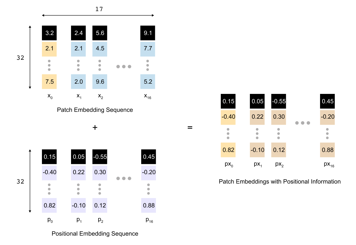
So after patch embedding and adding the class token we have a sequence of N+1 tokens, each of dimension D. We collect them in a matrix X, where x_0 is the class token and x1,…,x_N are the patch embeddings. The Vision Transformer introduces a learnable positional embedding matrix
where each row p_i is a trainable vector that represents the position of token i. During training these vectors are updated like any other parameter in the model. For a mini batch of size B we broadcast the same positional matrix over the batch and form the final input to the encoder by simple elementwise addition
The tensor sent into the transformer encoder therefore has shape B×(N+1)×D. The sequence length and embedding size are unchanged, but each token now carries two kinds of information at once: the visual content of its patch and the location of that patch in the original grid.
1.4 Encoder-only structure for classification
In a Vision Transformer we only keep the encoder side of the original transformer architecture. The image is converted into a sequence of tokens and these tokens pass through a stack of L identical encoder blocks. Each block contains multi-head self attention, a feed-forward MLP, and residual connections with layer normalization, but there is no decoder that predicts future tokens. Instead, we prepend a single learnable class token to the sequence and treat the encoder as a feature extractor. After the last encoder block we read out only the final hidden state of this class token and feed it into a small MLP head that produces the class logits for the image. In this sense a ViT is an encoder-only model trained for classification.
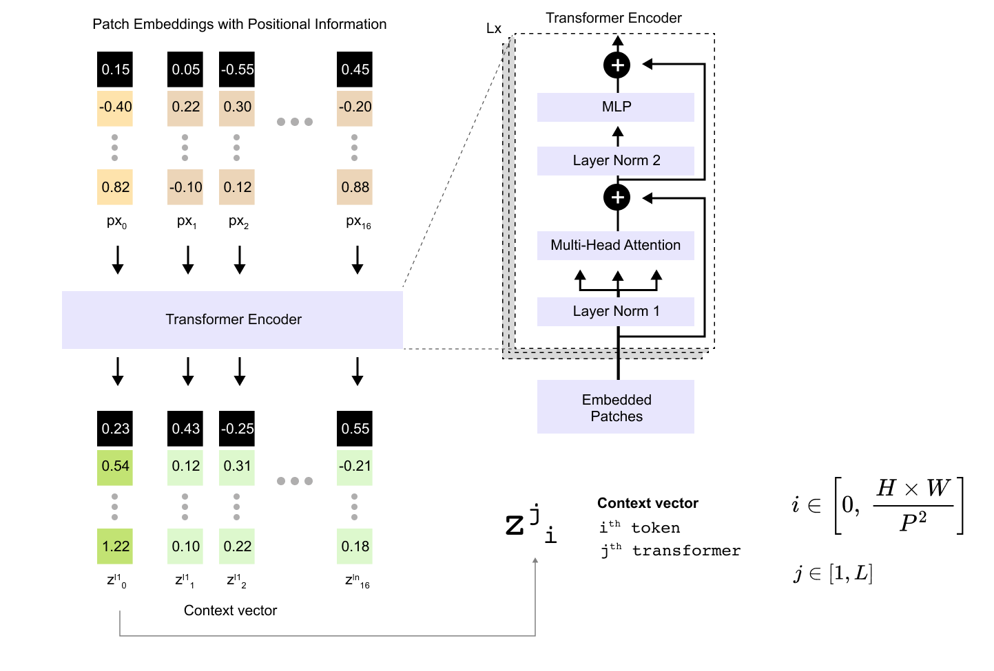
The entire path from patch embeddings to context vectors
From the previous sections we already have a matrix of embedded tokens that combines patch information and positional information. We then add one extra token for classification, so the total sequence length is N+1. Each token has embedding dimension D. If we stack all token vectors row wise we obtain a matrix
With the class token we therefore have N+1= 17 tokens. If we choose an embedding dimension D=32, the matrix E has shape 17×32. This matrix is the input to the transformer encoder stack and from the encoder’s perspective it looks exactly like the token embeddings of a language model: a batch of sequences, each of length 17, each token represented by a 32-dimensional vector.
The encoder does not change the sequence length. After each encoder block we still have a matrix of shape (N+1)×D, but every row vector has been updated to incorporate information from all other tokens through self attention and the MLP. These updated vectors are what we call context vectors, because they encode both the content of a token and the context supplied by the other tokens in the sequence.
Transformer encoder and attention
To understand what happens inside one encoder block it is helpful to zoom into the self-attention sublayer. At the input of a block we have a matrix
where j denotes the depth of the block in the stack. The rows of this matrix are the current representations of the tokens. Self attention transforms this matrix into a new matrix of the same shape by letting every token look at every other token and decide how much to pay attention to it.
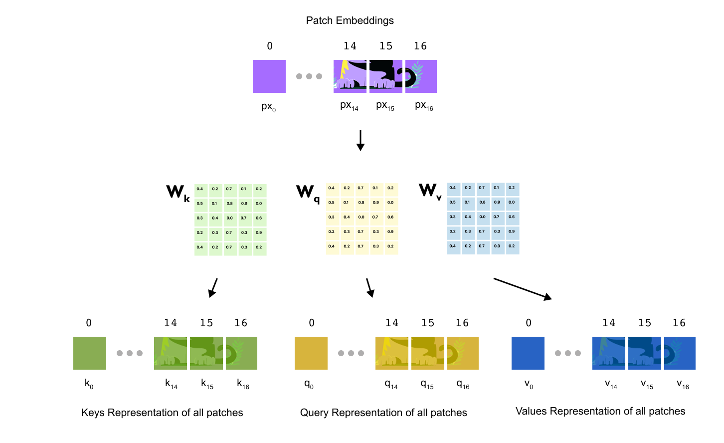
The first step is to project the token representations into three new spaces called queries, keys and values. Concretely, we multiply Z^(j) by three learnable weight matrices
where d_h is the head dimension for a single attention head. These weight matrices are shared across all positions in the sequence and are learned during training. Applying them gives three new matrices
each of shape (N+1)×dh. Intuitively, the query vector q_i for token i encodes what that token is looking for in its context, the key vector k_i encodes what that token offers to others, and the value vector v_i encodes the actual information that will be blended into other tokens when they attend to it.
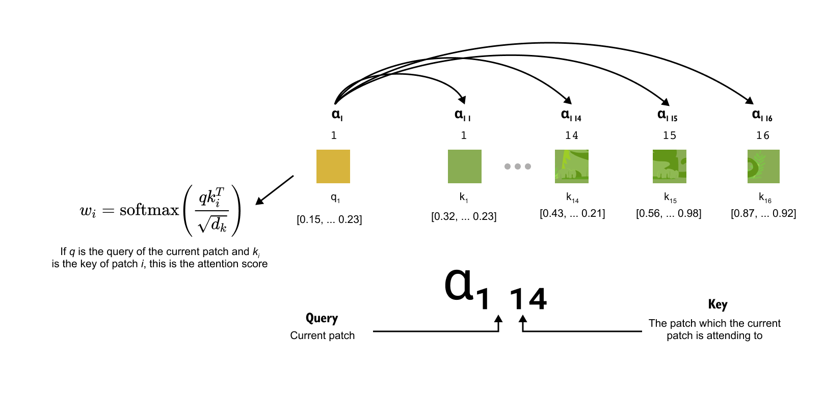
The second step is to turn queries and keys into attention weights. For a given query vector q_i we compute its similarity with every key k_j using a scaled dot product, which produces a scalar score for each pair of positions
The softmax function along the index j converts these scores into a probability distribution
so that
The coefficient α_ij can be read as “how much token i attends to token j”
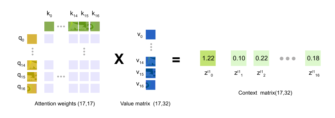
The third step is to use these attention weights to blend the value vectors. For token i we take a weighted sum of all values
The vector
is the new representation of token i produced by this attention head. It contains a mixture of the value vectors of all tokens, with larger weights coming from positions that were judged more relevant by the scaled dot product. If a head learns to focus on the cat’s eye, for example, the value vectors from patches around the eye will receive larger coefficients when computing the context vector for the class token.
In practice a Vision Transformer uses multi-head attention rather than a single head. This means we repeat the procedure above several times in parallel with different sets of projection matrices
Each head has its own head dimension d_h, so after computing
for every head we concatenate the results and use another learned projection to return to the original embedding dimension D. This gives the attention sublayer output matrix of shape (N+1)×D, which is then passed through the MLP sublayer and residual connections to form the updated matrix
Context vectors and output dimensions
To keep track of how representations evolve through the encoder stack, it is useful to introduce a simple notation. Let
be the initial matrix of token embeddings after patch embedding and positional embedding. After the j-th encoder block we write
where
is the context vector for token i at depth j. The index i runs from 0 to N. When i=0 the vector corresponds to the class token. When i ≥ 1 it corresponds to one of the image patches. Because the encoder stack never changes the sequence length, every Z^(j) has exactly the same shape: (N+1)×D. For our 640×640 cat image with P=160 and D=32 that means each encoder block takes a 17×32 matrix as input and produces another 17×32 matrix as output.
After the final encoder block we obtain Z^(L). The most important vector in this matrix is z_0^(L), the last context vector of the class token. During training this vector has learned to aggregate information from all patch tokens through the repeated layers of self attention and MLPs. As a result it acts as a compact summary of the entire image. We feed z_0^(L) into a small MLP head that maps the D-dimensional vector to a vector of class logits, for example of dimension 1000 for ImageNet-1k. A softmax over these logits then gives a probability distribution over classes.

MLP head and classification
By the time the sequence has passed through the transformer encoder, all of the heavy lifting has already happened. Starting from our cat image, we created N = 16 patch tokens, added a single learnable class token at the beginning, and mapped everything into a D-dimensional embedding space. After L encoder blocks, we obtain the final sequence matrix
Each row
is a context vector for token i, where i=0 corresponds to the class token and i = 1,…,N correspond to the image patches. In our running toy example N+1=17 and D=32 , so Z^(L) has shape 17×32
For image classification we do not feed all seventeen context vectors into a separate network. Instead, we follow the original ViT design and use only the final context vector of the class token,
This vector has attended to every patch token at every encoder layer, so it acts as a learned summary of the entire image. Using a single summary vector keeps the architecture simple and keeps the number of parameters in the final classifier small. In principle one could pool or concatenate all patch context vectors, but this would increase the dimensionality of the classifier input and did not bring clear benefits in the ViT experiments.
The MLP head is an ordinary feed-forward classifier that takes
as input and outputs one logit for each class. In the simplest case it consists of a single linear layer with weight matrix
and bias vector
where C is the number of labels (for example, cat, dog, bird, and so on). The logits vector is then
Many practical ViT implementations insert a small two-layer MLP here instead of a single linear layer. In that case we first project
to a hidden dimension D_mlp, apply a nonlinearity such as GELU, optionally apply dropout for regularisation, and then project down to C dimensions. The overall effect is to give the classifier a bit more capacity to reshape the representation coming from the transformer encoder before turning it into class scores.
The output y is a vector of unnormalised scores, or logits, one per class. At inference time we usually take the index of the largest logit as the predicted label. During training we pass y through a softmax to obtain a probability distribution over classes and compute a cross-entropy loss against the true label. Gradients from this loss flow back through the MLP head into the transformer encoder and further into the patch and positional embeddings, allowing the entire Vision Transformer to be trained end to end.
1.5 Benefits and drawbacks of ViT
Vision Transformers offer a conceptually clean and flexible alternative to convolutional networks by modeling images as sequences of tokens and relying entirely on self-attention to capture relationships between image regions. One of their key strengths is global context modeling: from the very first encoder layer, every image patch can attend to every other patch. This makes ViTs particularly effective at capturing long-range dependencies, such as relationships between distant parts of an object or interactions between foreground and background regions. In addition, the ViT architecture scales extremely well with data and model size. When trained on large-scale datasets, Vision Transformers often surpass convolutional networks in accuracy, showing that explicit convolutional inductive biases are not strictly necessary when sufficient data is available. Their architectural simplicity is another advantage: apart from the patch embedding stage, the model closely mirrors standard transformer encoders used in language models, making it easy to reuse ideas, optimizations, and tooling across vision and language domains.
However, these benefits come with important trade-offs. Vision Transformers are generally less data-efficient than convolutional networks, especially on small or medium-sized datasets. Without the strong locality and translation-equivariance biases of convolutions, ViTs must learn many visual regularities directly from data, which can lead to poorer performance when training data is limited. Self-attention also introduces higher computational and memory costs, as attention scales quadratically with the number of patches. For high-resolution images, this can quickly become a bottleneck. As a result, many practical ViT variants introduce hierarchical structures, windowed attention, or hybrid CNN–Transformer designs to mitigate these issues. In short, Vision Transformers excel when data and compute are abundant, but require careful design choices to remain competitive in more constrained settings.
1.6 Real-World Applications of Vision Transformers
Vision Transformers are now widely used across a broad range of real-world vision tasks, particularly in settings where large datasets and pretraining are available. In image classification, ViTs and their variants have become strong alternatives to deep convolutional networks, achieving state-of-the-art performance on large benchmarks when pretrained on massive image collections and fine-tuned on downstream tasks. Beyond classification, Vision Transformers have proven highly effective in object detection and image segmentation, where global context is especially valuable. Tasks such as detecting small objects in cluttered scenes or segmenting large, spatially distributed structures benefit from the ability of self-attention to relate distant patches directly.
In industrial and applied domains, Vision Transformers are increasingly used in medical imaging, remote sensing, and autonomous systems. In medical imaging, ViTs help model complex spatial relationships in high-resolution scans, such as MRI or histopathology images, where long-range dependencies can be diagnostically important. In satellite and aerial imagery, they are used for land-use classification, change detection, and large-scale scene understanding. Vision Transformers are also central to modern multimodal systems, where images must be aligned with text, audio, or other modalities. Models such as image–text encoders rely on ViT backbones to produce visual representations that integrate naturally with language transformers. As a result, Vision Transformers have become a foundational component in systems for image captioning, visual question answering, and large multimodal models, reinforcing their role as a unifying architecture across perception tasks.
1.7 Hands-on: fine-tuning ViT for image classification
Finetuning Vision Transformer Code Repo Link available below
https://github.com/VizuaraAI/Transformers-for-vision-BOOK
In this section we fine-tune a pretrained Vision Transformer on a real-world, high-resolution image classification task. The Oxford-IIIT Pet dataset provides sufficiently detailed visual structure to match the inductive biases of Vision Transformers, making it an ideal dataset for demonstrating practical ViT fine-tuning. We adapt a ViT-Base model pretrained on ImageNet and fine-tune it to classify pet images into breed categories, following a standard transfer-learning workflow used in modern vision systems.
Dataset and problem setup

The Oxford-IIIT Pet Dataset consists of 7,349 images of cats and dogs across 37 fine-grained breed classes. Images vary in resolution but are typically larger than 200×200 pixels and contain rich texture, shape, and spatial cues. Each image is labeled with a single breed, making this a multiclass classification problem. Although the dataset images are already reasonably high-resolution, pretrained Vision Transformers expect inputs of size 224×224, so we standardize all images to this resolution during preprocessing.
This dataset is a good fit for demonstrating ViT fine-tuning for several reasons:
Fine-grained categories. Distinguishing between 37 pet breeds requires the model to attend to subtle visual differences in fur pattern, ear shape, and body proportion, exactly the kind of long-range spatial reasoning that self-attention handles well.
Sufficient visual complexity. The images contain natural backgrounds, varying poses, and different lighting conditions, giving the model a realistic transfer learning challenge.
Manageable size. With roughly 3,680 training images and 3,669 test images, the dataset is small enough to fine-tune on a single GPU in reasonable time, yet large enough to produce meaningful results.
Installing dependencies and setting constants
Before we write any model code, we install the required libraries and define the hyperparameters that will stay fixed throughout the experiment:
Listing 1.1 Installing dependencies and defining constants
!pip install torchmetrics -q
import torch
import torch.nn as nn
import torch.optim as optim
import matplotlib.pyplot as plt
import numpy as np

from torchvision import datasets, transforms
from torch.utils.data import DataLoader
from transformers import ViTForImageClassification, ViTImageProcessor
from transformers import get_cosine_schedule_with_warmup

from torchmetrics.classification import MulticlassAccuracy
from sklearn.metrics import confusion_matrix, ConfusionMatrixDisplay

from tqdm.auto import tqdm
device = torch.device("cuda" if torch.cuda.is_available() else "cpu")
torch.manual_seed(42)
torch.cuda.manual_seed_all(42)
NUM_CLASSES = 37
IMAGE_SIZE = 224
BATCH_SIZE = 32
EPOCHS = 50We fix the random seed so that results are reproducible, and we set NUM_CLASSES = 37 to match the 37 pet breeds in the Oxford-IIIT dataset. The image size of 224 matches the resolution that the pretrained ViT-Base model expects.
Loading and exploring the dataset
We use torchvision.datasets.OxfordIIITPet to download and load the dataset. The dataset provides both a train-val split (used for training) and a test split (used for validation):
Listing 1.2 Loading the Oxford-IIIT Pet dataset
raw_train = datasets.OxfordIIITPet(
    root="./data",
    split="trainval",
    target_types="category",
    download=True
)

class_names = raw_train.classes
print(len(class_names))
print(class_names[:10])
this prints
37
['Abyssinian', 'Bengal', 'Birman', 'Bombay', 'British_Shorthair',
'Egyptian_Mau', 'Maine_Coon', 'Persian', 'Ragdoll', 'Russian_Blue']
Visualizing sample images
This listing displays a small grid of pet images to highlight the dataset’s visual diversity and resolution.
Listing 1.3 Visualizing sample images from the dataset
plt.figure(figsize=(12, 6))

for i in range(8):
    img, label = raw_train[i]
    plt.subplot(2, 4, i + 1)
    plt.imshow(img)
    plt.title(class_names[label])
    plt.axis("off")

plt.show()
output
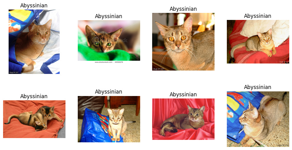
From this visualization we observe that images contain rich textures, variable poses, and complex backgrounds. These properties make long-range attention over image patches particularly valuable.
Preprocessing and data loaders
Pretrained Vision Transformers are sensitive to the normalization statistics used during pretraining. We load the ViTImageProcessor to extract the correct mean and standard deviation, and then build separate transforms for training and validation:
Listing 1.4 Building preprocessing pipelines with ViTImageProcessor
processor = ViTImageProcessor.from_pretrained(
"google/vit-base-patch16-224"
)
print(processor)
Output
ViTImageProcessor {
  "do_convert_rgb": null,
  "do_normalize": true,
  "do_rescale": true,
  "do_resize": true,
  "image_mean": [
    0.5,
    0.5,
    0.5
  ],
  "image_processor_type": "ViTImageProcessor",
  "image_std": [
    0.5,
    0.5,
    0.5
  ],
  "resample": 2,
  "rescale_factor": 0.00392156862745098,
  "size": {
    "height": 224,
    "width": 224
  }
}
image_mean = processor.image_mean
image_std = processor.image_std

train_transforms = transforms.Compose([
    transforms.RandomResizedCrop(IMAGE_SIZE),
    transforms.RandomHorizontalFlip(),
    transforms.ToTensor(),
    transforms.Normalize(mean=image_mean, std=image_std)
])

val_transforms = transforms.Compose([
    transforms.Resize(IMAGE_SIZE),
    transforms.CenterCrop(IMAGE_SIZE),
    transforms.ToTensor(),
    transforms.Normalize(mean=image_mean, std=image_std)
])
The training transforms apply random resized cropping and horizontal flipping for data augmentation, while the validation transforms use a deterministic resize and center crop so that evaluation is reproducible. Both pipelines normalize using the ImageNet statistics that the pretrained model was trained with.
After preprocessing, every image has shape
which matches the ViT input specification.
We now construct the training and validation datasets and wrap them in PyTorch DataLoaders.
Listing 1.5 Constructing training and validation data loaders
train_dataset = datasets.OxfordIIITPet(
    root="./data",
    split="trainval",
    target_types="category",
    transform=train_transforms
)

val_dataset = datasets.OxfordIIITPet(
    root="./data",
    split="test",
    target_types="category",
    transform=val_transforms
)

train_loader = DataLoader(train_dataset, batch_size=BATCH_SIZE, shuffle=True)
val_loader = DataLoader(val_dataset, batch_size=BATCH_SIZE, shuffle=False)
Loading the pretrained model
We load a ViT-Base model pretrained on ImageNet using the Hugging Face transformers library. The key argument num_labels=NUM_CLASSES tells the library to replace the original 1000-class ImageNet head with a new linear head that outputs 37 logits,one per pet breed.
The ignore_mismatched_sizes=True flag suppresses the warning about the size mismatch in the classification head:
Listing 1.6 Loading a pretrained ViT-Base model with a new classification head
model = ViTForImageClassification.from_pretrained(
    "google/vit-base-patch16-224",
    num_labels=NUM_CLASSES,
    ignore_mismatched_sizes=True
).to(device)
print(model)The output model structure would be
ViTForImageClassification(
  (vit): ViTModel(
    (embeddings): ViTEmbeddings(
      (patch_embeddings): ViTPatchEmbeddings(
        (projection): Conv2d(3, 768, kernel_size=(16, 16), stride=(16, 16))
      )
      (dropout): Dropout(p=0.0, inplace=False)
    )
    (encoder): ViTEncoder(
      (layer): ModuleList(
        (0-11): 12 x ViTLayer(
          (attention): ViTAttention(
            (attention): ViTSelfAttention(
              (query): Linear(in_features=768, out_features=768, bias=True)
              (key): Linear(in_features=768, out_features=768, bias=True)
              (value): Linear(in_features=768, out_features=768, bias=True)
            )
            (output): ViTSelfOutput(
              (dense): Linear(in_features=768, out_features=768, bias=True)
              (dropout): Dropout(p=0.0, inplace=False)
            )
          )
          (intermediate): ViTIntermediate(
            (dense): Linear(in_features=768, out_features=3072, bias=True)
            (intermediate_act_fn): GELUActivation()
          )
          (output): ViTOutput(
            (dense): Linear(in_features=3072, out_features=768, bias=True)
            (dropout): Dropout(p=0.0, inplace=False)
          )
          (layernorm_before): LayerNorm((768,), eps=1e-12, elementwise_affine=True)
          (layernorm_after): LayerNorm((768,), eps=1e-12, elementwise_affine=True)
        )
      )
    )
    (layernorm): LayerNorm((768,), eps=1e-12, elementwise_affine=True)
  )
  (classifier): Linear(in_features=768, out_features=37, bias=True)
)
Freezing the backbone and training only the head
A common transfer-learning strategy is to freeze all pretrained parameters and train only the newly initialized classification head. This is fast, requires little memory, and often produces strong results when the pretrained features already capture the visual concepts needed for the target task:
Listing 1.7 Freezing the backbone and counting trainable parameters
for param in model.parameters():
    param.requires_grad = False
for name, param in model.named_parameters():
    if "classifier" in name:
       param.requires_grad = True
We can verify the freeze with a quick parameter count:
def print_model_parameters(model):
    trainable_params = 0
    frozen_params = 0
    all_param = 0

    for _, param in model.named_parameters():
        num_params = param.numel()
        all_param += num_params

        if param.requires_grad:
            trainable_params += num_params
        else:
            frozen_params += num_params

    print(f"trainable params: {trainable_params:,}")
    print(f"frozen params:    {frozen_params:,}")
    print(f"all params:       {all_param:,}")
    print(f"trainable%:       {100 * trainable_params / all_param:.2f}%")

# Run the function
print_model_parameters(model)
The output shows that only the classification head is trainable, roughly 28,000 parameters out of the model’s 86 million total:
trainable params: 28,453
frozen params: 85,798,656
all params: 85,827,109
trainable%: 0.03%
Sanity check: pre-training inference
Before any fine-tuning, we run the model on a single validation image to establish a baseline. Since the classification head is randomly initialized, we expect the prediction to be essentially random:
Listing 1.8 Sanity check: pre-training inference on one image
model.eval()

image, label = val_dataset[0]
image = image.unsqueeze(0).to(device)

with torch.no_grad():
    outputs = model(pixel_values=image)
    logits = outputs.logits
    probs = torch.softmax(logits, dim=1)
    pred = probs.argmax(dim=1).item()
    confidence = probs.max(dim=1).values.item()

print(
    f"[Pre-training inference]\n"
    f"  Ground truth class : {class_names[label]}\n"
    f"  Predicted class    : {class_names[pred]}\n"
    f"  Prediction confidence : {confidence:.2f}"
)
Output
[Pre-training inference]
  Ground truth class : Abyssinian
  Predicted class    : Shiba Inu
  Prediction confidence : 0.05
The model predicts an incorrect class with low confidence, confirming that the head needs training.
Setting up the optimizer, scheduler, and loss
We use AdamW with a learning rate of 3 × 10⁻⁴ and a cosine schedule with linear warmup. The warmup phase helps stabilize early training when the head weights are still random:
Listing 1.9 Setting up AdamW optimizer, cosine scheduler, and loss function
optimizer = optim.AdamW(
    filter(lambda p: p.requires_grad, model.parameters()),
    lr=3e-4,
    weight_decay=1e-4
)


total_steps = len(train_loader) * EPOCHS
warmup_steps = int(0.1 * total_steps)

scheduler = get_cosine_schedule_with_warmup(
    optimizer,
    num_warmup_steps=warmup_steps,
    num_training_steps=total_steps
)

criterion = nn.CrossEntropyLoss()
accuracy = MulticlassAccuracy(num_classes=NUM_CLASSES).to(device)
AdamW for fine-tuning
AdamW is a variant of Adam that decouples weight decay from the gradient update. This prevents the regularization from interfering with the adaptive learning rate, leading to better generalization. It is the standard optimizer for both pretraining and fine-tuning transformers.
The training loop
The training loop follows a standard PyTorch pattern: for each epoch, iterate over mini-batches, compute the cross-entropy loss, back-propagate, and update the classification-head weights. After each epoch, we evaluate on the validation set:
Listing 1.10 The main training and validation loop
train_losses, val_accuracies = [], []

for epoch in range(EPOCHS):
    model.train()
    running_loss = 0.0

    for imgs, labels in tqdm(train_loader):
        imgs, labels = imgs.to(device), labels.to(device)

        outputs = model(pixel_values=imgs)
        loss = criterion(outputs.logits, labels)

        optimizer.zero_grad()
        loss.backward()
        optimizer.step()
        scheduler.step()

        running_loss += loss.item()

    train_losses.append(running_loss / len(train_loader))

    model.eval()
    accuracy.reset()
    with torch.no_grad():
        for imgs, labels in val_loader:
            imgs, labels = imgs.to(device), labels.to(device)
            preds = model(pixel_values=imgs).logits.argmax(dim=1)
            accuracy.update(preds, labels)

    val_accuracies.append(accuracy.compute().item())

    print(f"Epoch {epoch+1}: "
          f"Loss={train_losses[-1]:.4f}, "
          f"Val Acc={val_accuracies[-1]:.4f}")
Note how we call model.train() at the start of each epoch to enable dropout and batch-norm updates, and model.eval() before validation to disable them. The scheduler.step() call happens after each optimizer step (not each epoch), which is the correct behavior for the cosine-with-warmup schedule.
Plotting training progress
After training, we plot the training loss and validation accuracy curves to assess convergence:
Listing 1.11 Plotting training loss and validation accuracy curves
plt.figure(figsize=(12, 4))

plt.subplot(1, 2, 1)
plt.plot(train_losses)
plt.title("Training Loss")
plt.xlabel("Epoch")
plt.ylabel("Loss")

plt.subplot(1, 2, 2)
plt.plot(val_accuracies)
plt.title("Validation Accuracy")

plt.xlabel("Epoch")
plt.ylabel("Accuracy")
plt.tight_layout()
plt.show()
Output plot
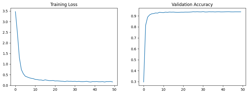
A healthy run will show the training loss decreasing steadily and the validation accuracy climbing over the first several epochs before leveling off. Since we are only training the classification head, convergence is typically fast.
Post-training inference
We can now verify that the fine-tuned model makes correct predictions on validation images:
Listing 1.12 Post-training inference on a validation image
model.eval()

image, label = val_dataset[0]
image = image.unsqueeze(0).to(device)

with torch.no_grad():
    logits = model(pixel_values=image).logits
    pred = logits.argmax(dim=1).item()

print("After training → Pred:", class_names[pred],
      "| GT:", class_names[label])
Output
After training → Pred: Abyssinian | GT: AbyssinianConfusion matrix evaluation
To understand where the model excels and where it struggles, we compute a confusion matrix over the entire validation set. This reveals which breed pairs are most easily confused:
Listing 1.13 Computing and displaying the confusion matrix
all_preds, all_labels = [], []

model.eval()
with torch.no_grad():
    for imgs, labels in val_loader:
        imgs = imgs.to(device)
        # Get predictions
        preds = model(pixel_values=imgs).logits.argmax(dim=1)

        all_preds.extend(preds.cpu().numpy())
        all_labels.extend(labels.numpy())

cm = confusion_matrix(all_labels, all_preds)
disp = ConfusionMatrixDisplay(cm, display_labels=class_names)


fig, ax = plt.subplots(figsize=(30, 30))

disp.plot(ax=ax, xticks_rotation=45, colorbar=True)


plt.tight_layout()

plt.show()
Output
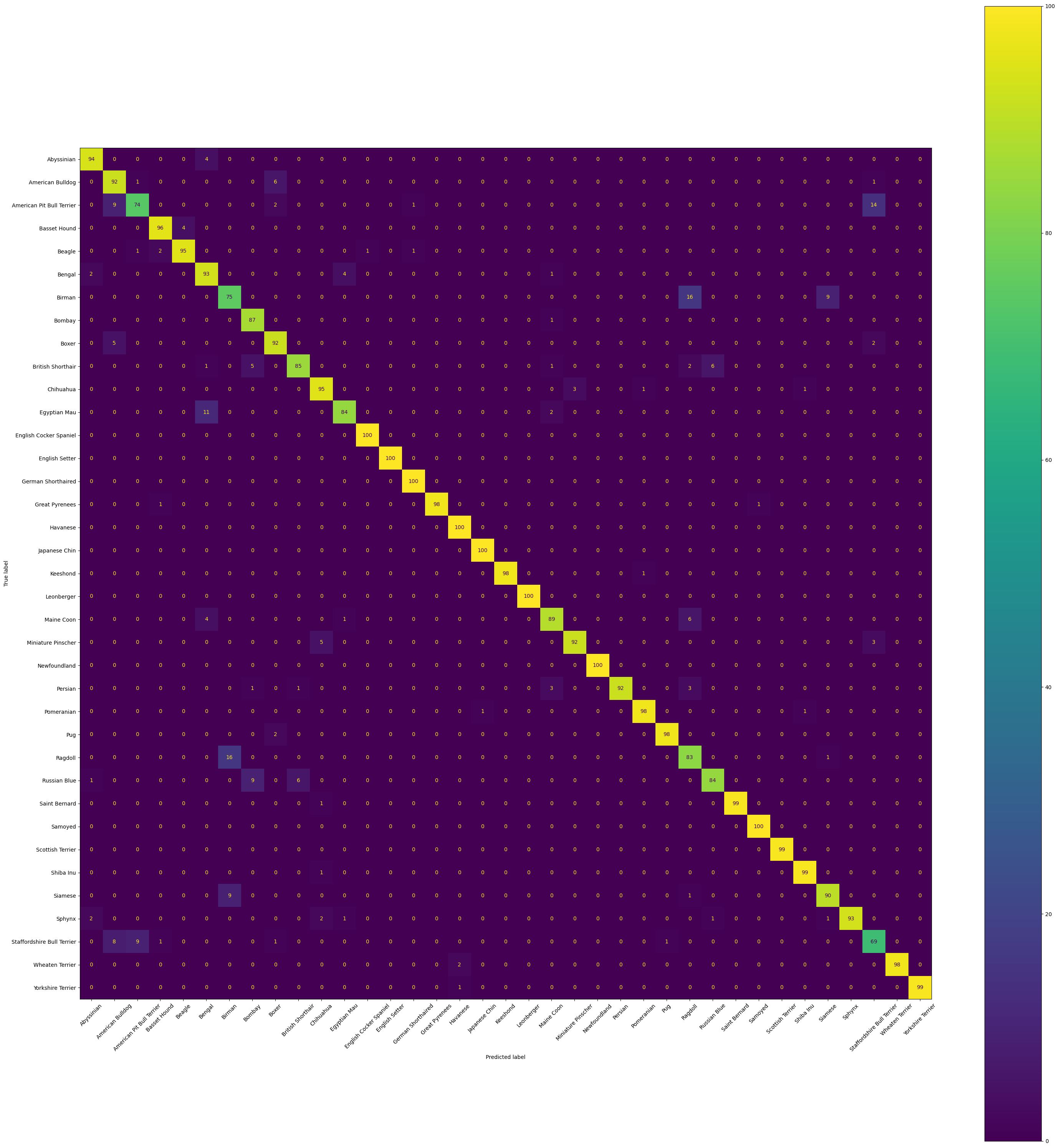
The diagonal entries show correct predictions; off-diagonal entries indicate confusions. Breeds with visually similar features (for example, different shorthaired cats) will typically show higher off-diagonal values. This kind of finegrained analysis is valuable for deciding whether to invest in more data, stronger augmentation, or a larger model.
Saving the fine-tuned model
Finally, we save the fine-tuned weights so that the model can be reloaded later for inference without retraining:
Listing 1.14 Saving the fine-tuned model weights
torch.save(model.state_dict(), "vit_finetuned_final.pth")
print("Model saved successfully.")
The .pth file contains only the model’s state_dict, a dictionary mapping each layer name to its parameter tensor. To reload the model, we would create a new ViTForImageClassification instance with the same configuration and call model.load_state_dict(torch.load("vit_finetuned_final.pth")).
Resources
Original Paper
An Image is Worth 16x16 Words: Transformers for Image Recognition at Scale
Dr Sreedath Panat
Vision Transformer Paper Dissection
Build Vision Transformer from Scratch
1.8 Summary
Vision Transformers adapt the transformer architecture to images by treating fixed-size image patches as tokens, enabling global self-attention from the first layer. Unlike convolutional networks, which build receptive fields gradually through stacked layers, ViTs can relate any two image regions directly.
Patch embedding converts a 2D image into a 1D sequence of token vectors. This can be done by flattening each patch and applying a linear projection, or equivalently by using a single convolution with kernel size and stride equal to the patch size.
A learnable class token is prepended to the sequence and accumulates information from all patches through self-attention. After the final encoder block, the class token’s context vector serves as a compact summary of the entire image and is passed to an MLP head for classification.
Learnable positional embeddings are added to each token so that the model retains spatial information about where each patch originated in the original image grid.
The encoder-only architecture processes the full patch sequence through L identical blocks of multi-head self-attention and feed-forward layers. Each block preserves the sequence length and embedding dimension, progressively refining token representations.
Vision Transformers scale well with large datasets and model sizes but are less data-efficient than CNNs on small datasets. Practical variants address the quadratic attention cost through hierarchical designs and windowed attention.
Fine-tuning a pretrained ViT on a downstream classification task follows a standard transfer-learning workflow: freeze the pretrained backbone, replace the classification head, and train only the head on the target dataset using a cosine learning rate schedule with warmup.
Some of More Substacks
I’m also building Audio Deep Learning projects and Exploring and Finetuning different tts,sst models, sharing and discussing them on LinkedIn and Twitter. If you’re someone curious about these topics, I’d love to connect with you all!
Mayank Pratap Singh
LinkedIn : www.linkedin.com/in/mayankpratapsingh022
Twitter/X : x.com/Mayank_022.