Understanding Self-Attention with Trainable Weights
K, Q, V intuition


Introduction
In this lecture from the Transformers for Vision series, we move beyond the simplified self-attention mechanism and step into the real engine that drives large language models like GPT - self-attention with trainable weights. In the earlier session, we computed attention scores simply by taking the dot product of input embeddings. While that gave us an intuitive foundation, it lacked one critical element that makes large models powerful - learning. Today, we will introduce the idea of trainable weight matrices associated with the key, query, and value vectors, and we will see why these matrices are essential in allowing a neural network to truly learn meaningful contextual relationships within a sequence.

Revisiting Simplified Self-Attention
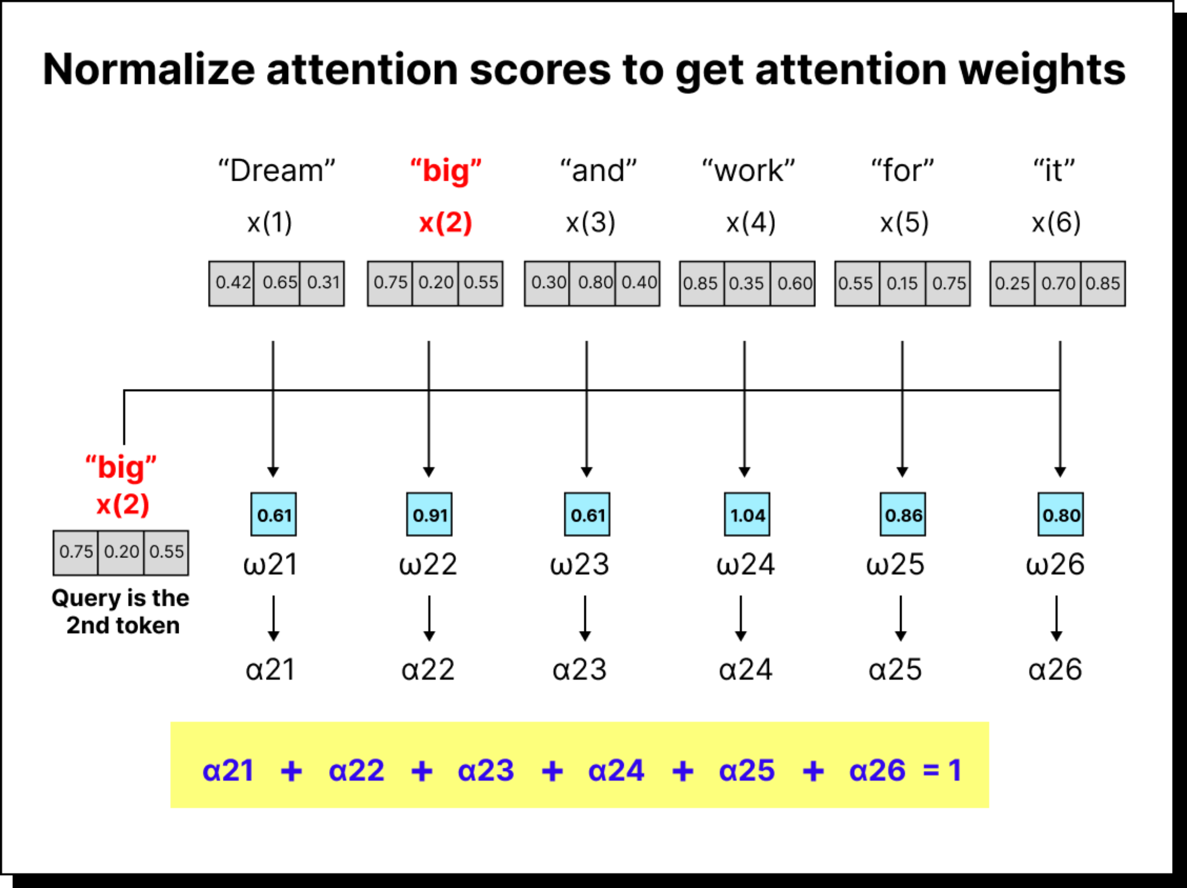
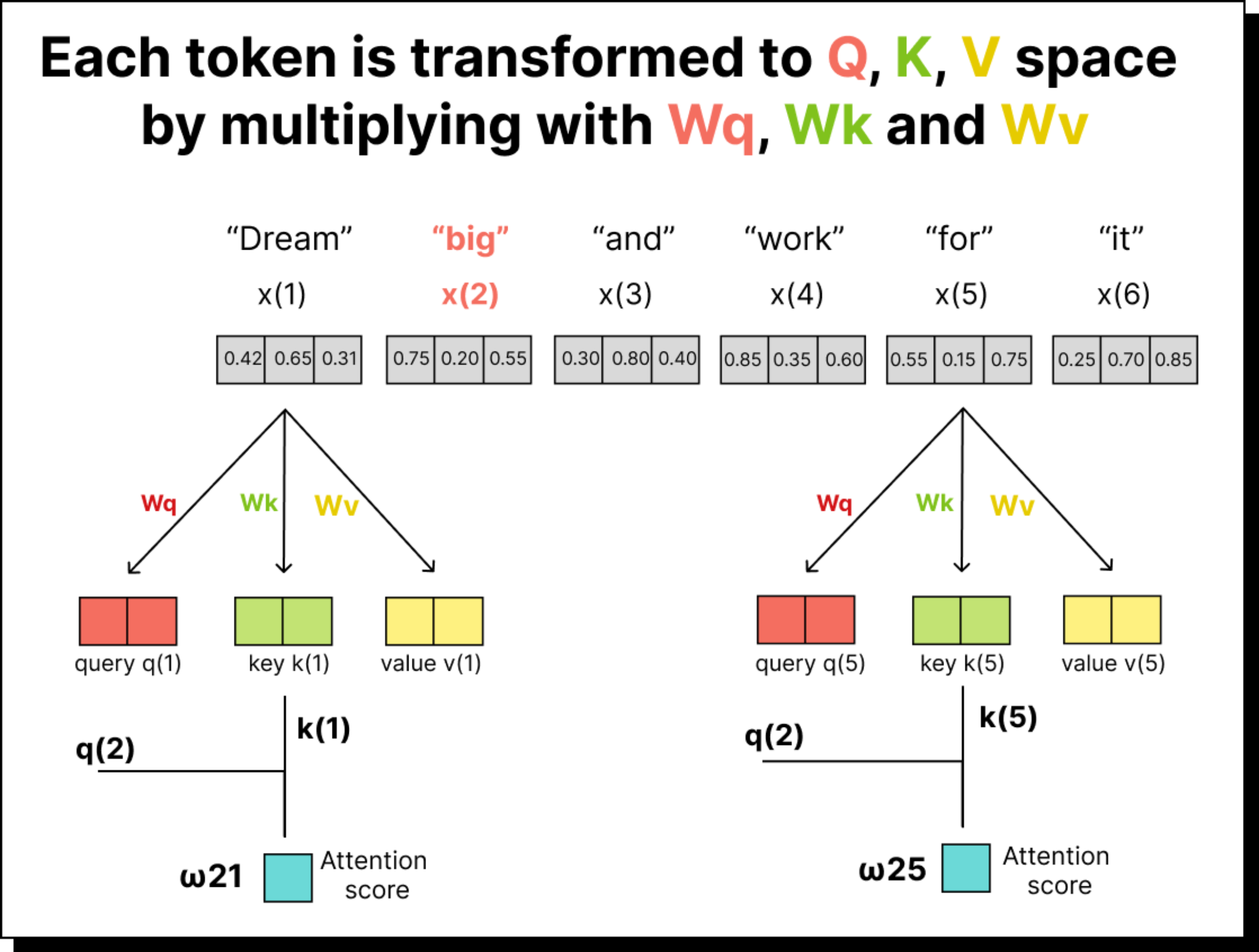
Before we jump into the details, let us take a moment to recall what we did earlier. In the simplified version of self-attention, we started with a sentence such as “dream big and work for it”. Each word was represented as an embedding vector in some multidimensional space. We took dot products between these vectors to measure similarity or alignment between them. For instance, the dot product between “big” and “dream” told us how much attention the token “big” should pay to “dream”. By repeating this for every pair of tokens and normalizing the results with a softmax function, we obtained what we called attention weights – numerical indicators of how much importance each word gives to every other word in the same sentence.
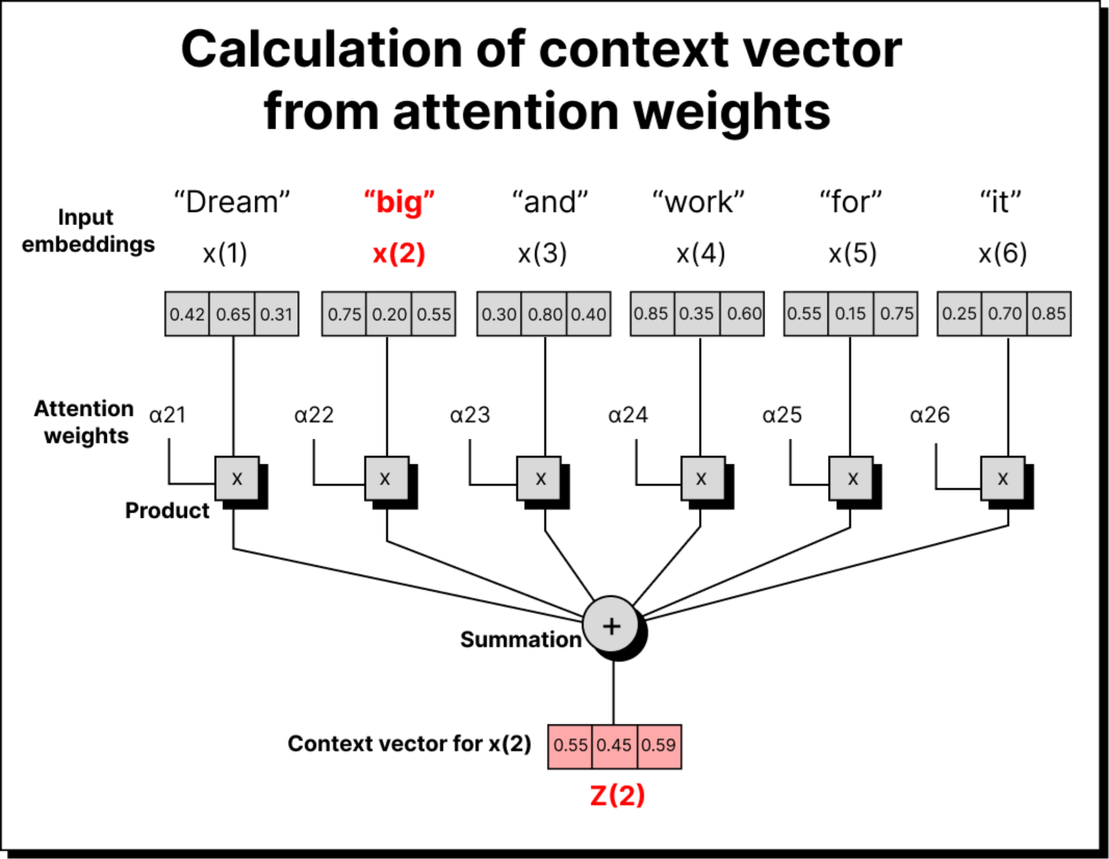
This method worked well for building intuition. It showed how context vectors can be constructed by taking weighted sums of other words’ embeddings. However, there was one big limitation – there were no trainable parameters involved. All the computations were based on fixed embeddings, and thus the model had no way to improve its understanding through learning.
The Limitation of Direct Dot Product
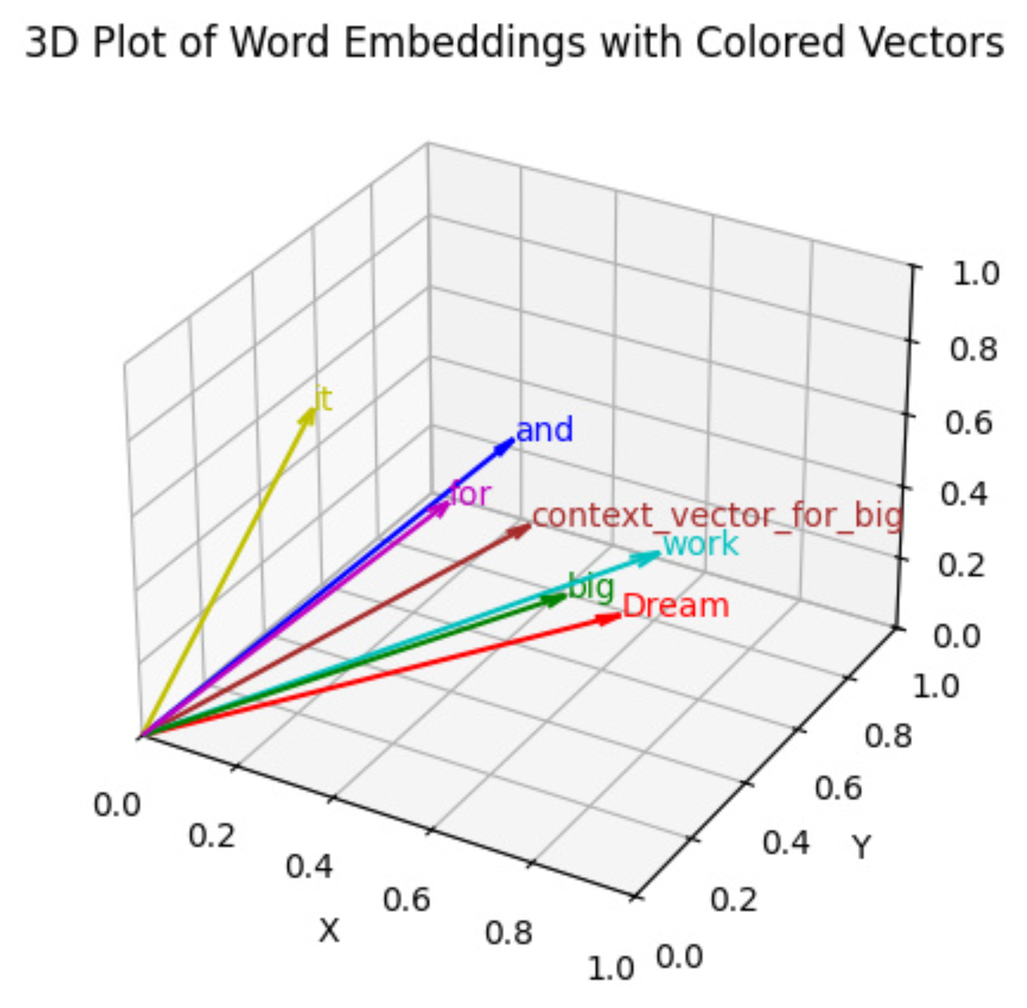
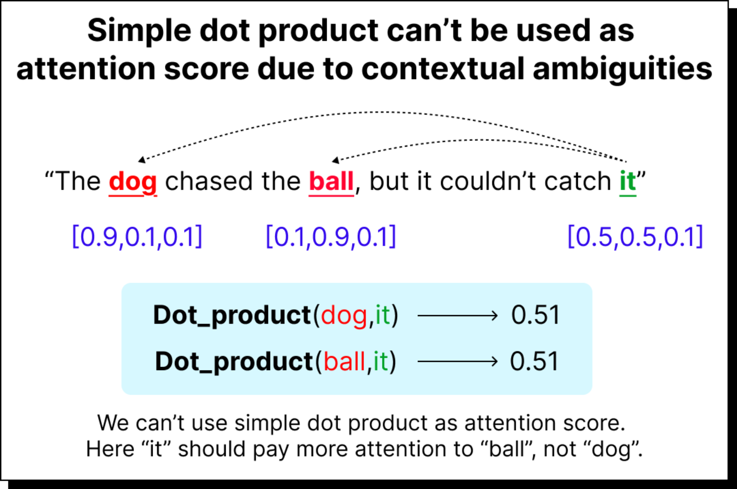
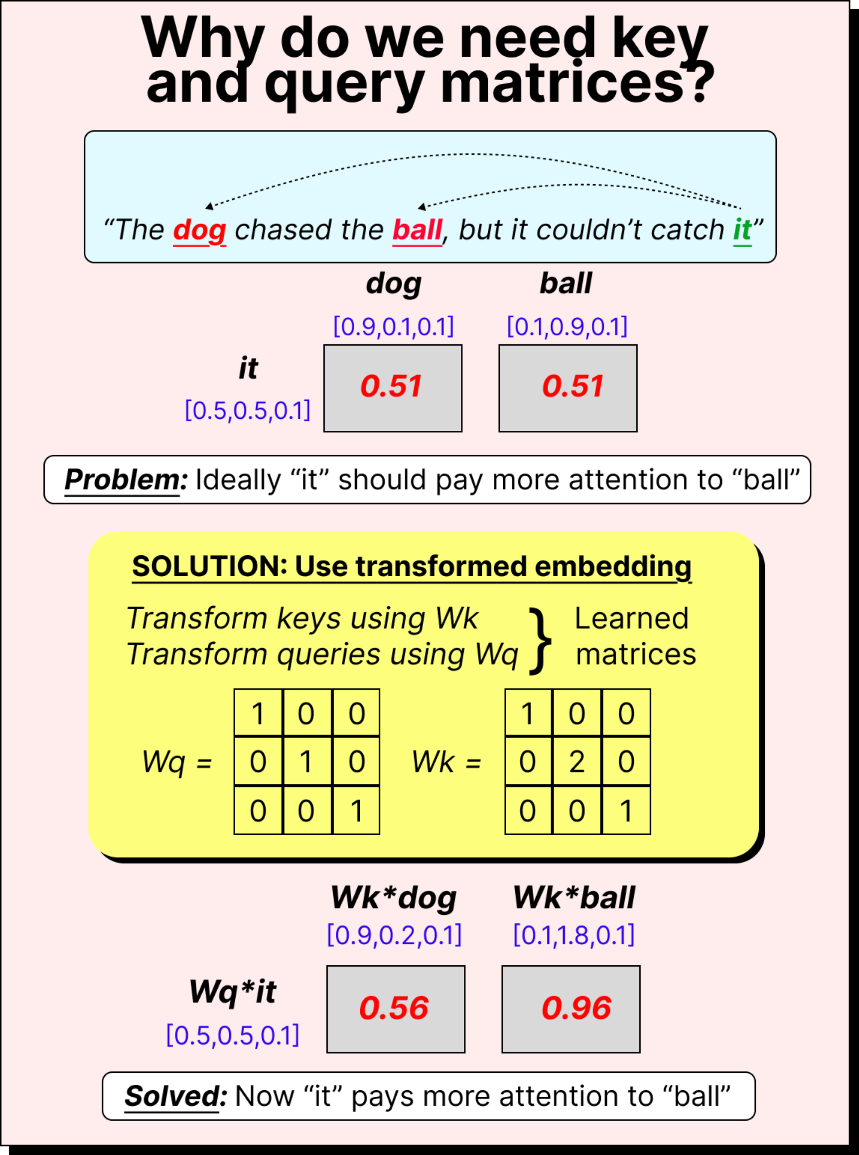
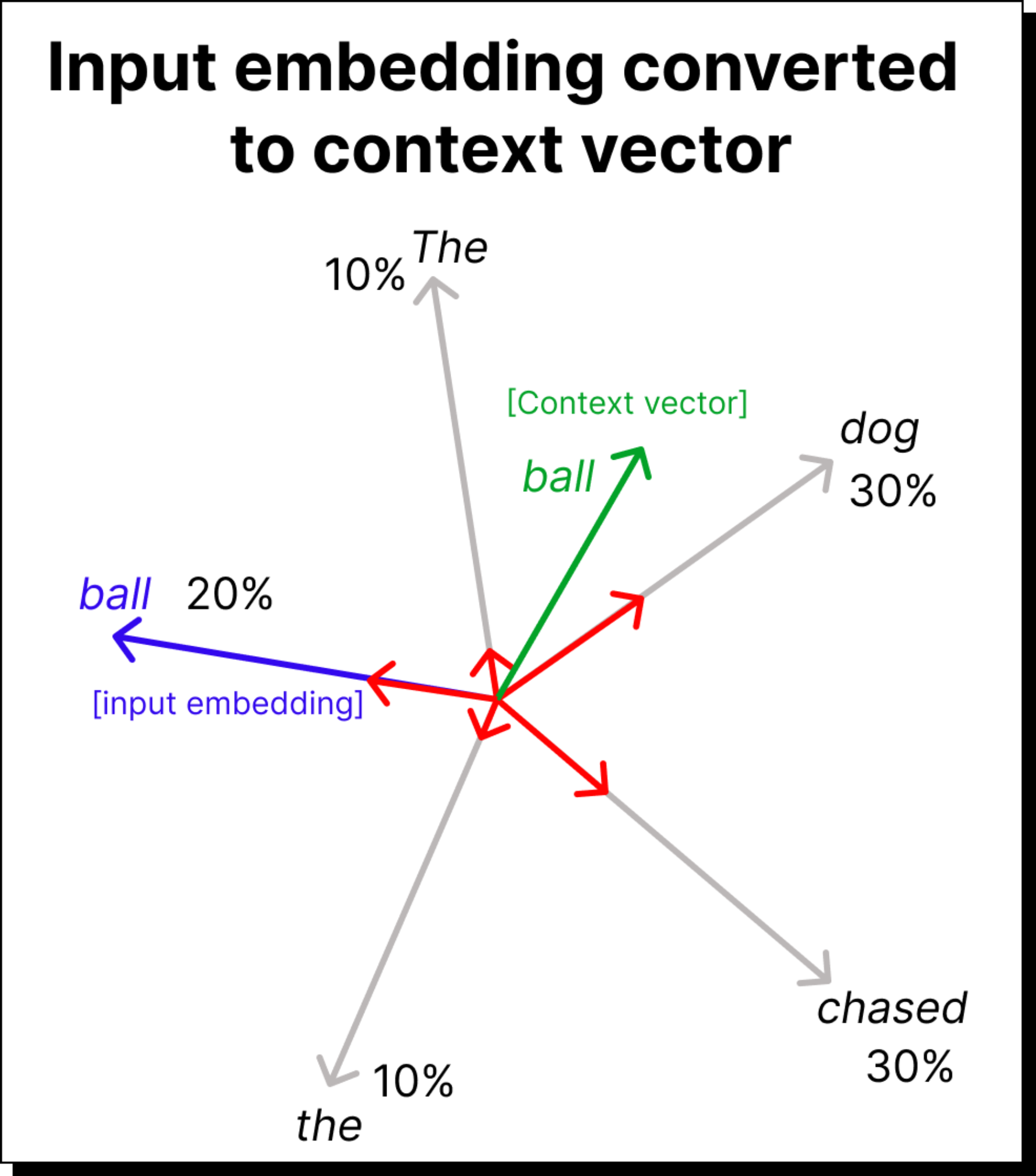
If you think about it carefully, simply taking dot products between fixed embeddings is not ideal. Although the direction of vectors captures semantic meaning (for instance, words pointing in similar directions tend to have related meanings), using raw embeddings can lead to poor attention behavior. Imagine a simple example with the sentence “The dog chased the ball, but it couldn’t catch it.” Here, the word “it” should ideally refer to “ball” rather than “dog”. But if we just take direct dot products of the embedding vectors, both pairs (it, ball) and (it, dog) might end up having similar attention scores. This means the attention mechanism would not be able to disambiguate which word “it” is referring to. Clearly, we need a way to transform these embeddings before taking their dot products.
Introducing the Trainable Weight Matrices
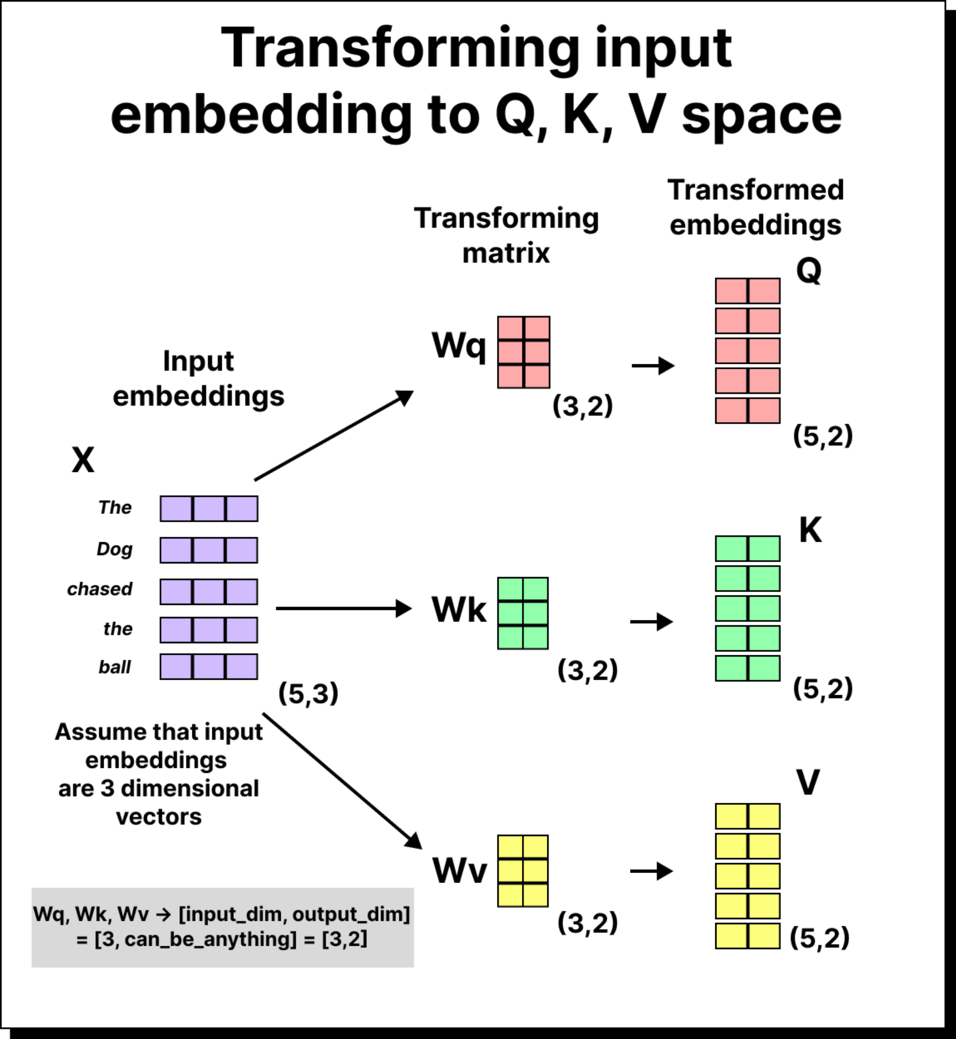
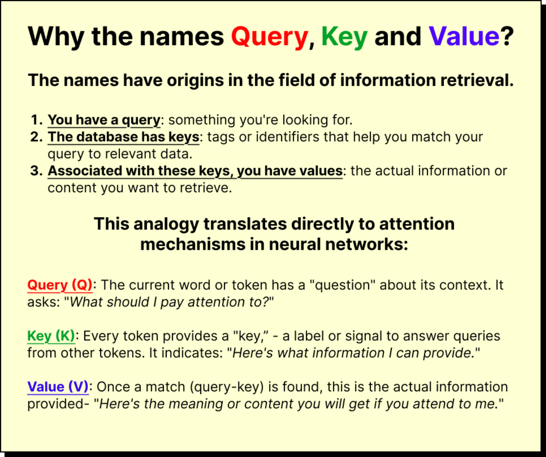
To solve this problem, the self-attention mechanism introduces three learnable matrices – WQ (query weight matrix), WK (key weight matrix), and WV (value weight matrix). Each of these matrices transforms the input embeddings into different representational spaces before we compute the dot products.
For example, if our sentence has five tokens and each token embedding is three-dimensional, the input matrix will be of size 5×3. When we multiply it with WQ (which might be of size 3×2), we get a 5×2 matrix – the transformed query vectors. The same process is repeated using WK and WV to obtain the key and value vectors. These matrices are trainable, meaning their values are learned and updated during training through backpropagation. Over time, the model learns transformations that allow it to capture subtle relationships between tokens.

Computing the Attention Scores
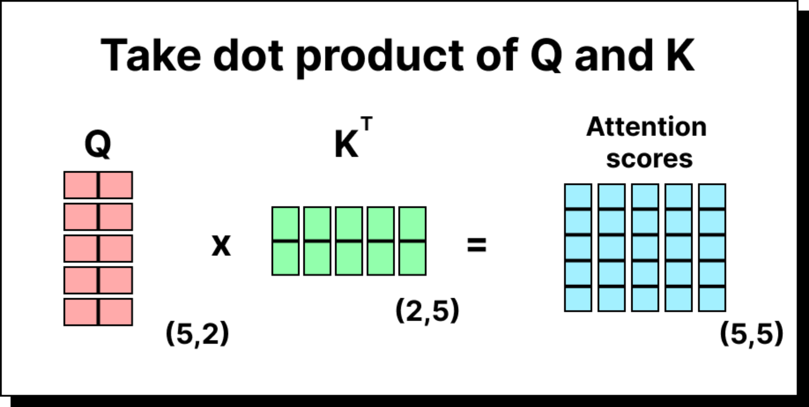
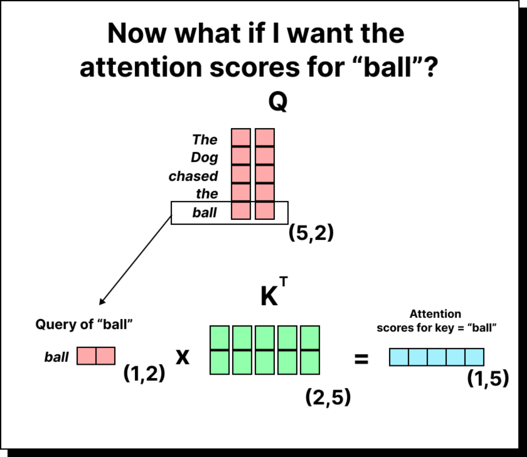
Once the embeddings are transformed, we can compute the attention scores by taking the dot product of queries with keys. If there are five tokens, we will have a 5×5 attention score matrix. Each entry in this matrix indicates how much one token (the query) attends to another token (the key). For instance, the entry in the second row and third column represents how much the second word should pay attention to the third word in the sequence.
However, these raw scores are not normalized. To convert them into meaningful probabilities, we apply two additional steps – scaling and softmax normalization.
The Need for Scaling
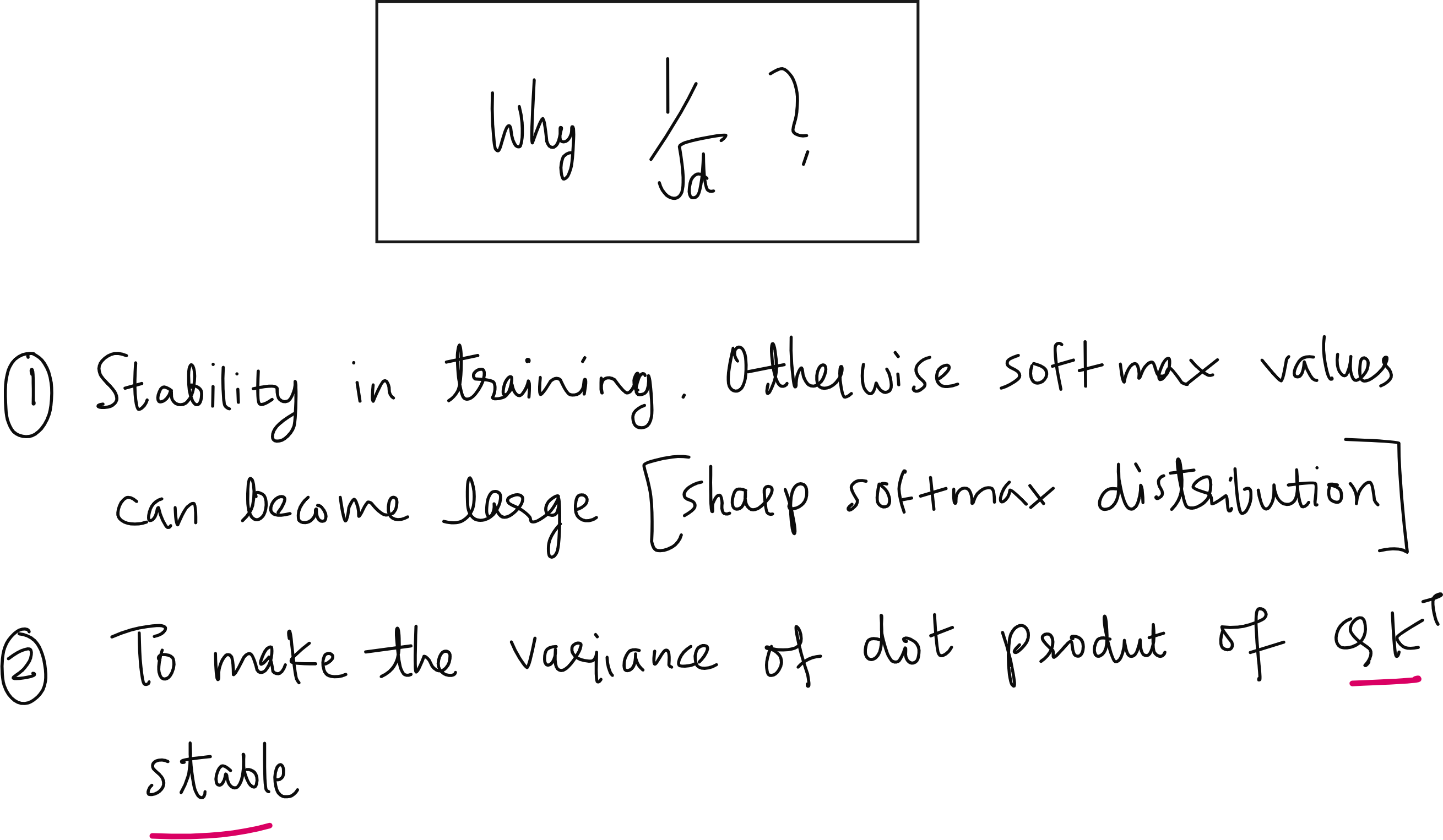
When the dimensionality of the key and query vectors is large, their dot product can yield very large values. Passing such large numbers directly into a softmax function can make it extremely sharp, meaning one token might receive almost all the attention while others get close to zero. This is not ideal for training stability or for proper gradient flow. To prevent this, the scores are divided by the square root of the dimension of the key space, denoted as √dₖ. This scaling ensures that the variance of the attention scores remains around 1 regardless of the dimensionality of the embeddings. It helps maintain stable training behavior even when the model is scaled up to hundreds of dimensions.
Softmax and Attention Weights
After scaling, the attention scores are passed through the softmax function. The result is a set of normalized attention weights that sum up to one. Each row of this matrix corresponds to a query token, and each column corresponds to how much that query pays attention to every key. These weights can now be interpreted as probabilities or relative importance scores.
Constructing the Context Vector Using Value Vectors
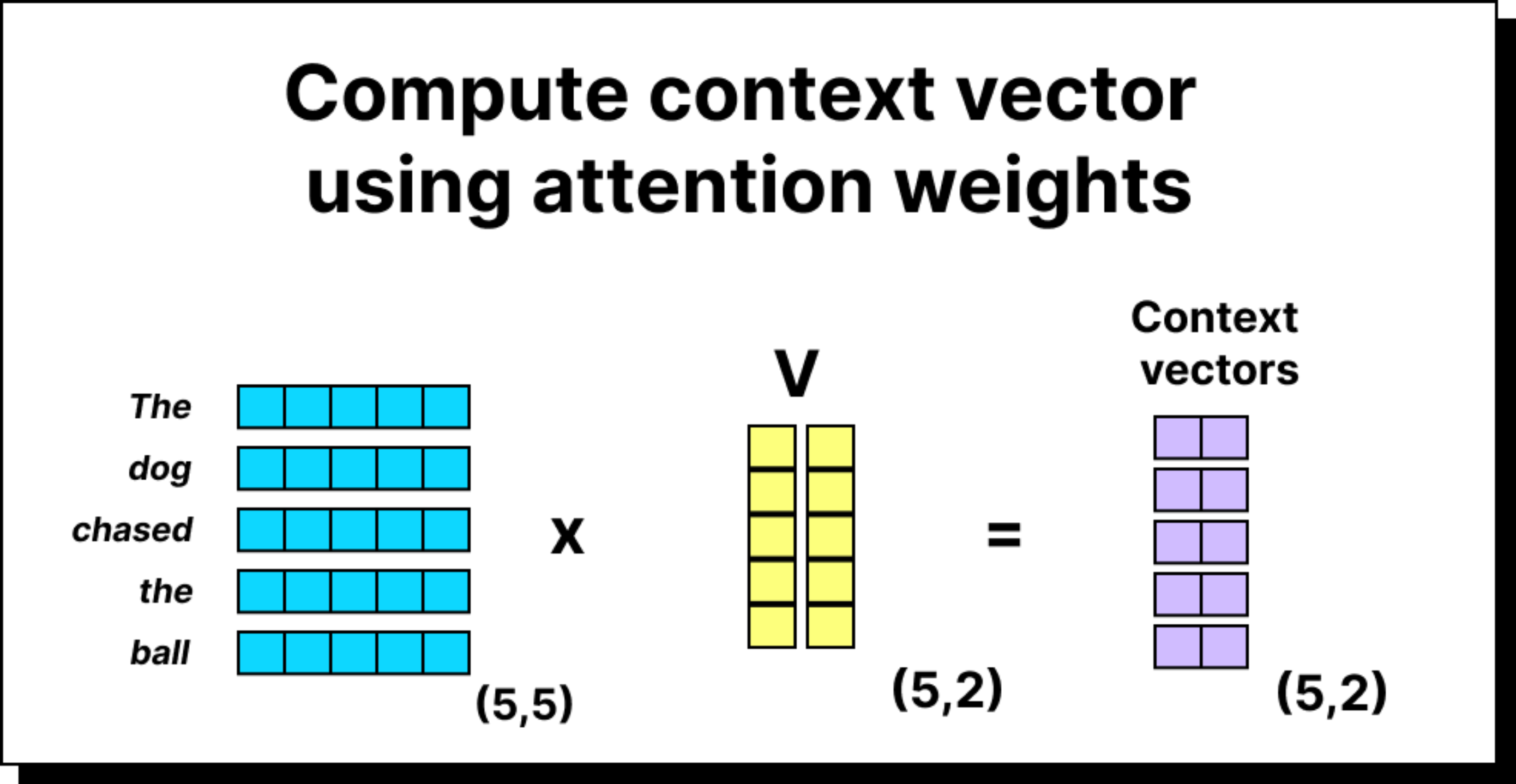
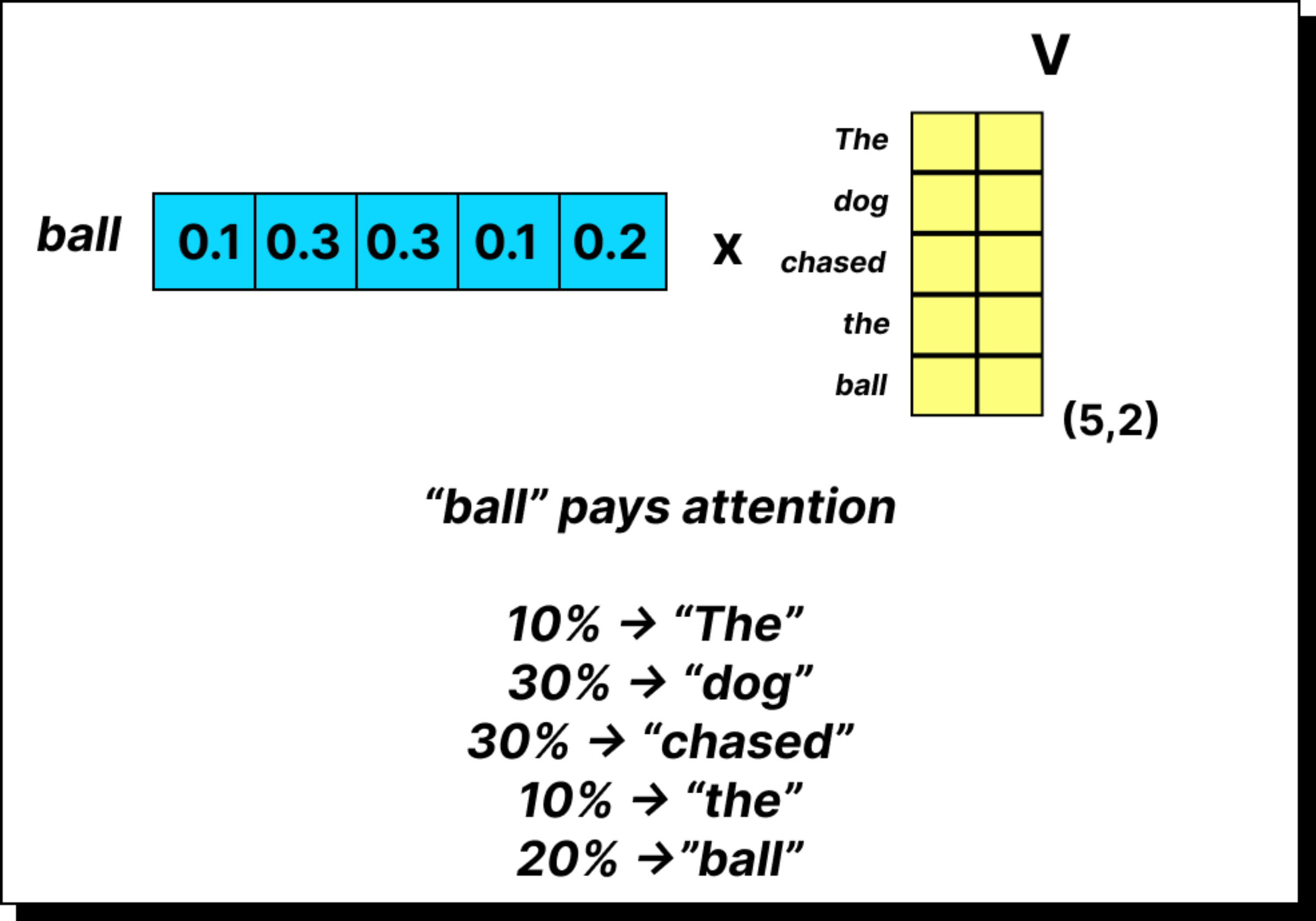
Now comes the final and most important step. Once we have the attention weights, we use them to compute the context vectors. In the simplified version, we multiplied the attention weights directly with the input embeddings. But in the complete self-attention mechanism, we multiply them with the value vectors, which are transformed embeddings obtained using the WV matrix. This gives us the weighted sum of the value vectors, where the weights come from the softmax attention scores. The result is a set of context vectors that encode information about both the token itself and its surrounding words. Each context vector now carries rich, contextualized meaning, which is far more useful to downstream layers of the model.
Why Divide by Square Root of d?
There are two main reasons for dividing by √d. The first is to prevent the softmax from becoming too sharp, as we discussed earlier. The second reason is related to variance stabilization. As the dimensionality of the vectors increases, the variance of the dot products also increases roughly in proportion to the dimension. Dividing by √d cancels out this effect, keeping the variance consistent across different dimensions. This makes training smoother and more reliable, regardless of how large the model is.
The Final Equation
With all these pieces in place, we can now understand the famous equation from the Attention is All You Need paper:
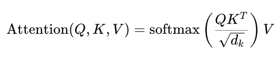
This equation neatly summarizes the entire process. We first transform the input embeddings into Q, K, and V using their respective trainable matrices. Then, we compute the dot product between Q and Kᵀ, scale it by √dₖ, apply softmax to get the attention weights, and finally multiply the result with V to get the context vectors.
Implementation Example
In the latter half of the lecture, we implemented this mechanism in code. Using a simple sequence such as “dream big and work for it”, we created random weight matrices for query, key, and value transformations using PyTorch. Each word embedding, originally in a three-dimensional space, was transformed into two-dimensional query, key, and value vectors. We computed the attention score matrix, applied scaling and softmax to get attention weights, and then used these weights to multiply the value vectors, obtaining the final context vectors. The resulting 6×2 matrix contained context-rich representations of each word.
Conclusion
The self-attention mechanism with trainable weights is the cornerstone of the transformer architecture. The introduction of the WQ, WK, and WV matrices allows the model to learn how to transform input embeddings into more meaningful spaces where relationships between tokens can be better captured. Through scaling, normalization, and weighted summation, the model produces context vectors that capture both local and global dependencies in a sequence. This is what enables transformers to understand long-range relationships and power state-of-the-art models in natural language processing, computer vision, and beyond.
Lecture video
PRO content: What will you get?