Understanding Principal Component Analysis

A must know technique in Machine Learning

Vizuara AI Labs

and

Sreedath Panat

May 05, 2025

There are two kinds of people in the world.

Those who reduce dimensions with PCA.
And those who actually understand what PCA is doing.

Most tutorials throw around phrases like “projects onto eigenvectors” and “maximizes variance” and then immediately import PCA from scikit-learn.

In this article, we are going to do something different. We will go from scratch.
From scatterplots to covariance matrices. From unit vectors to eigenvalues.
From theory to full code implementation in Julia.

Because if your understanding of PCA is only one function call deep, you are going to run into problems the moment your dataset misbehaves.

The intuition: Why PCA exists

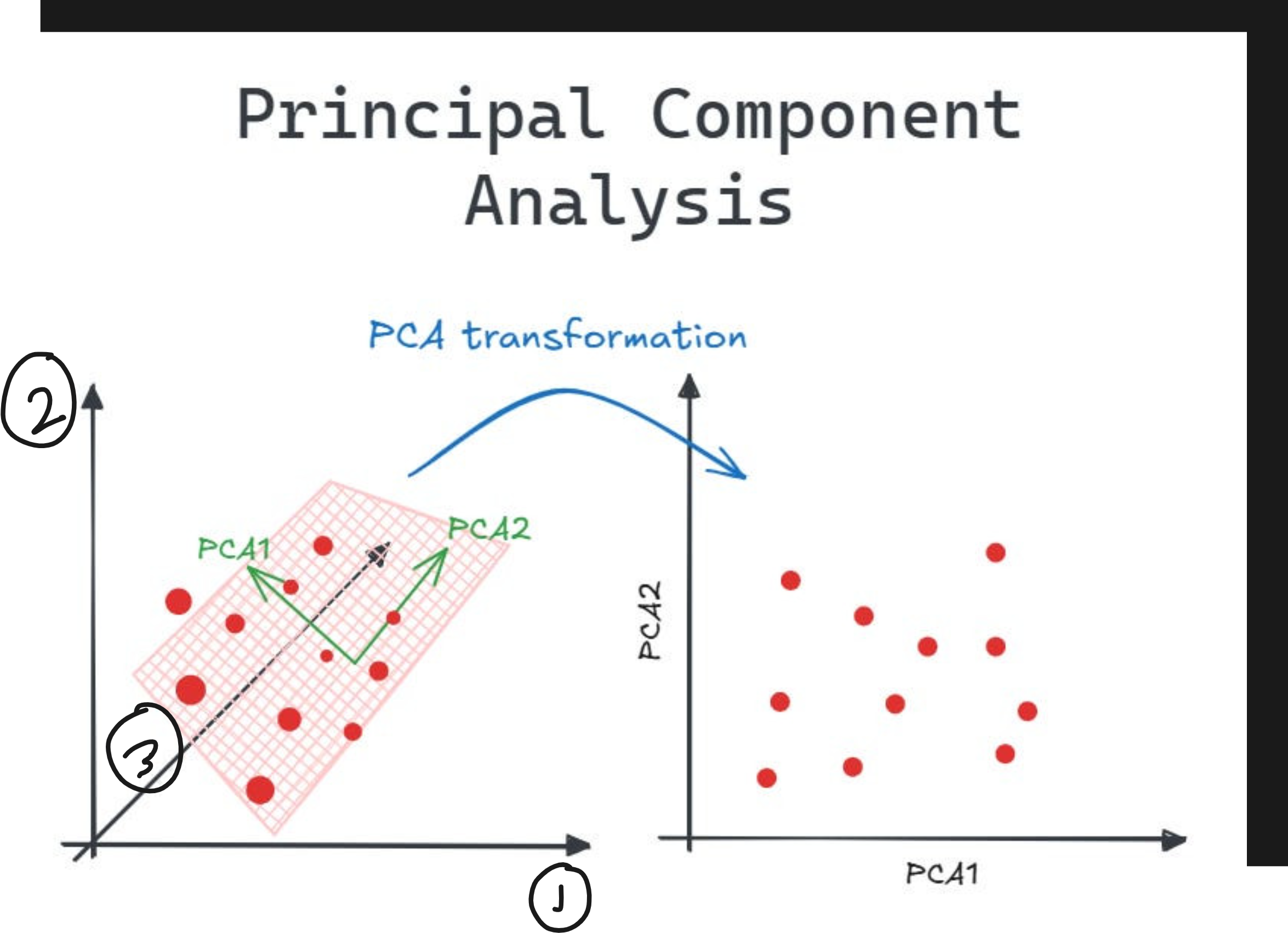
Imagine a 2D scatterplot of data. The points seem to follow a diagonal trend. One axis explains a lot. The other axis explains very little.

If you are trying to build a model, you do not need both axes. You can just rotate your coordinate system, project all points onto the line with maximum variance, and get a one-dimensional dataset that still preserves most of the information.

That is PCA in a sentence.

Instead of using your raw feature axes, PCA finds a new set of axes - the principal components - along which the data varies the most.
Then it lets you keep only the top k axes. You save space, reduce noise, and often improve model performance.

A Classification Example That Makes This Clear

Let us say you have a dataset with two features. You plot it and see two clusters - one red and one green - nicely separated along one axis.

Now imagine that the second axis has almost no spread. Even if you delete that axis entirely, the red and green points are still separable.

Congratulations. You just discovered that one of your features is redundant. PCA formalizes this insight and does it for hundreds of dimensions.

The Math: Step-by-Step, No Magic

Let us get technical. Suppose your dataset is the following.

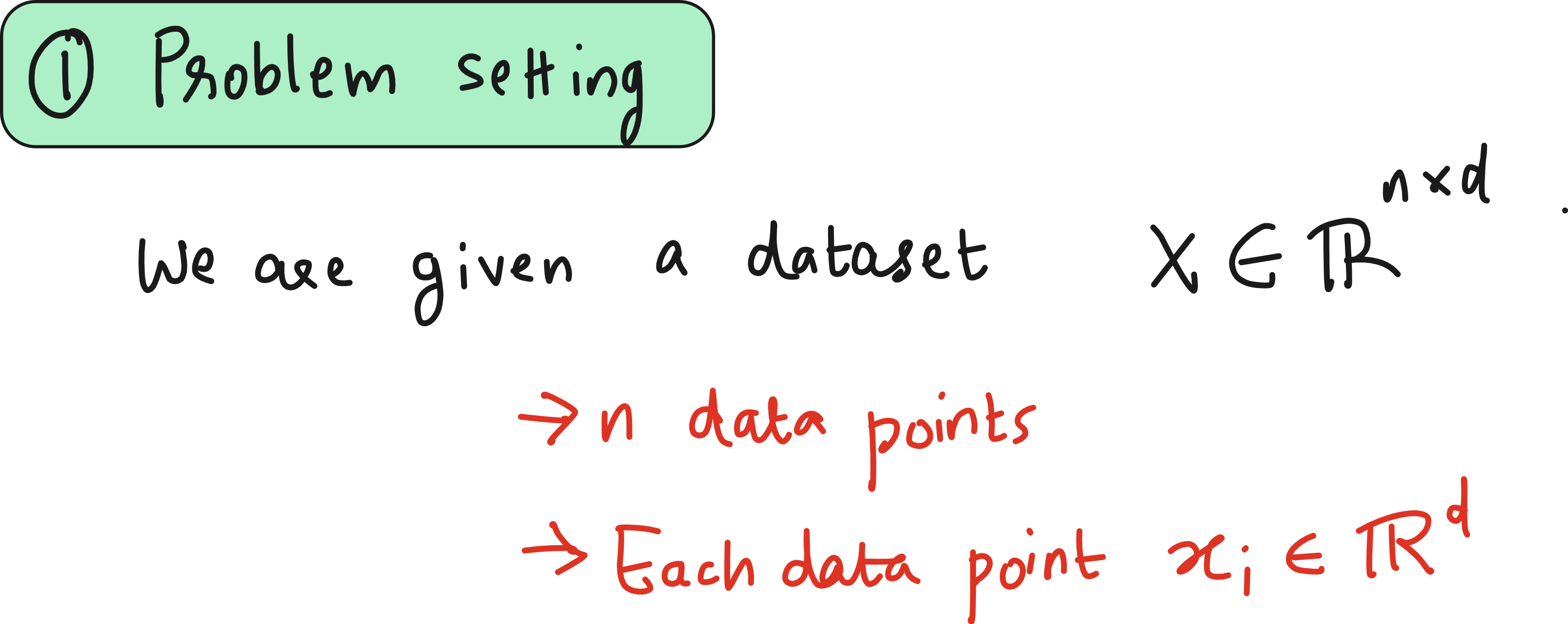
Step 1: Center the data
Subtract the mean across each feature. You want the dataset centered at the origin.
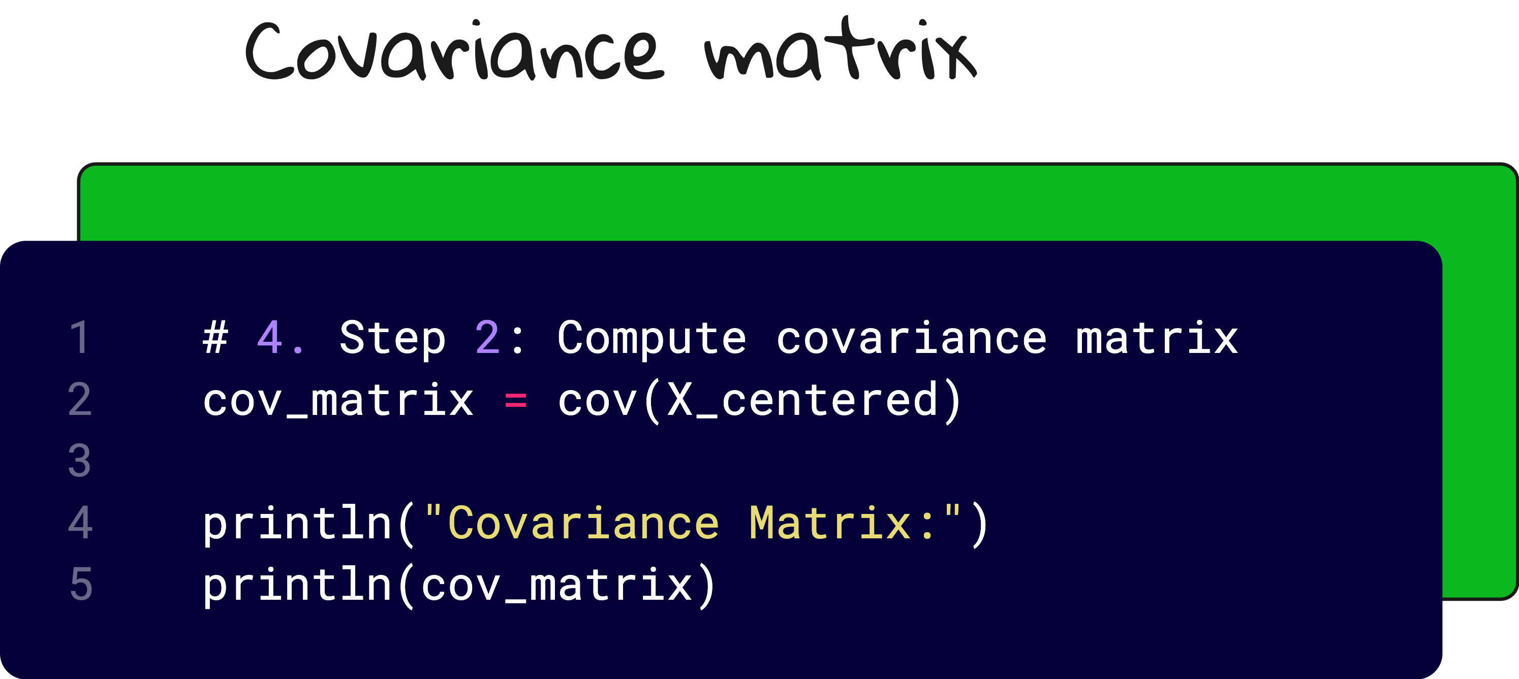
Step 2: Compute the covariance matrix
This tells you how different features co-vary. If two features are highly correlated, PCA will spot that.
Step 3: Define a direction
Take a unit vector w. Project each data point w. That projection is zi=w⊤xiz_i = w^\top x_izi=w⊤xi.
Step 4: Maximize the variance of z
.
Step 5: Use Lagrange Multipliers
This is the kicker: the direction that maximizes variance is an eigenvector of the covariance matrix.
The corresponding eigenvalue tells you how much variance you get along that direction.

So what are Principal Components?

The eigenvector with the largest eigenvalue is your first principal component. It captures the most variance.
The second eigenvector (orthogonal to the first) is the second principal component, and so on.

If your original dataset had d dimensions, and you only want to keep k, then you:

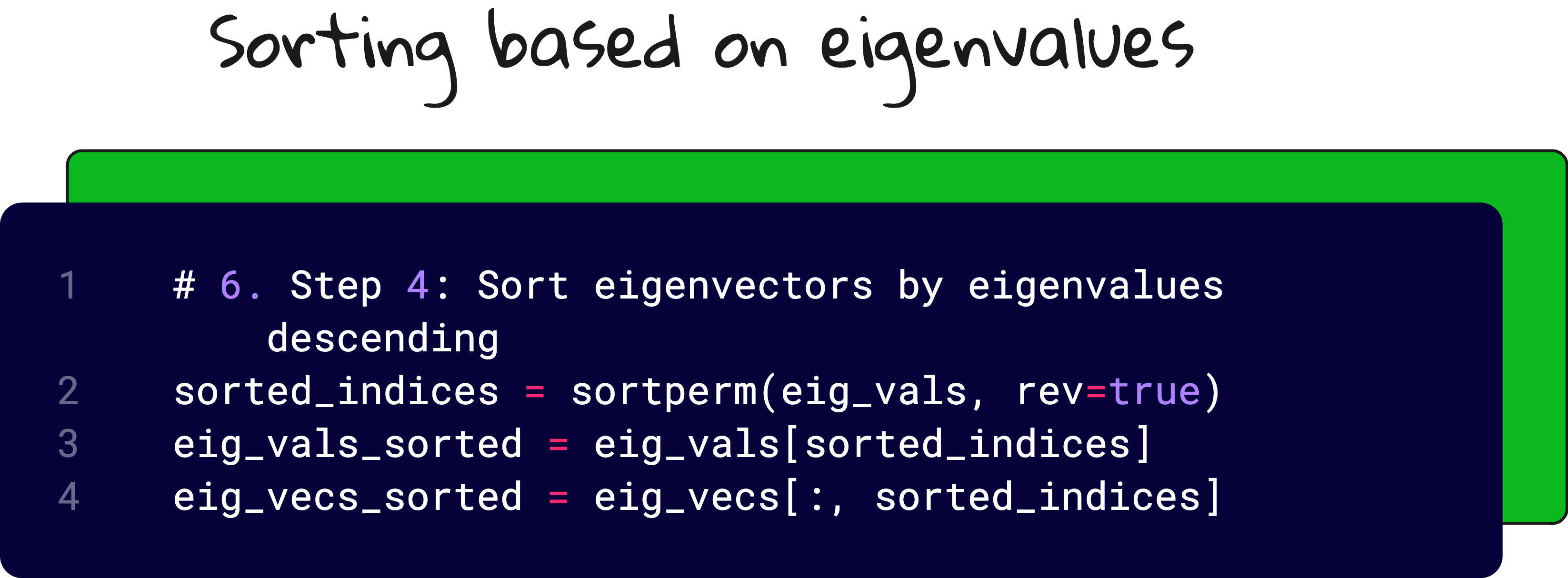
Sort the eigenvectors by their eigenvalues (descending)
Pick the top k
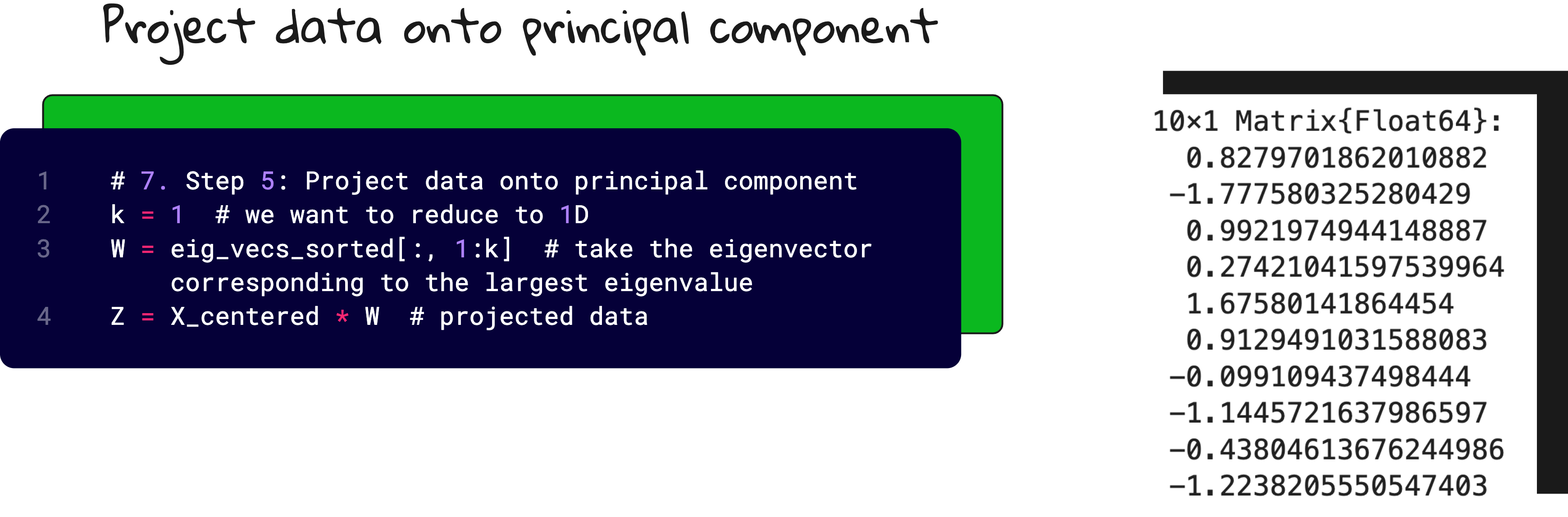
Project your data onto those vectors

Suddenly your n×d dataset becomes n×k.

Cleaner. Leaner. Easier to work with.

But theory is useless without code

I implemented the full PCA pipeline in Julia.

No high-level libraries. Just raw matrix operations, linear algebra, and plots.

You will:

Define a toy dataset
Center it
Compute the covariance matrix
Extract eigenvalues and eigenvectors
Sort them
Project the data
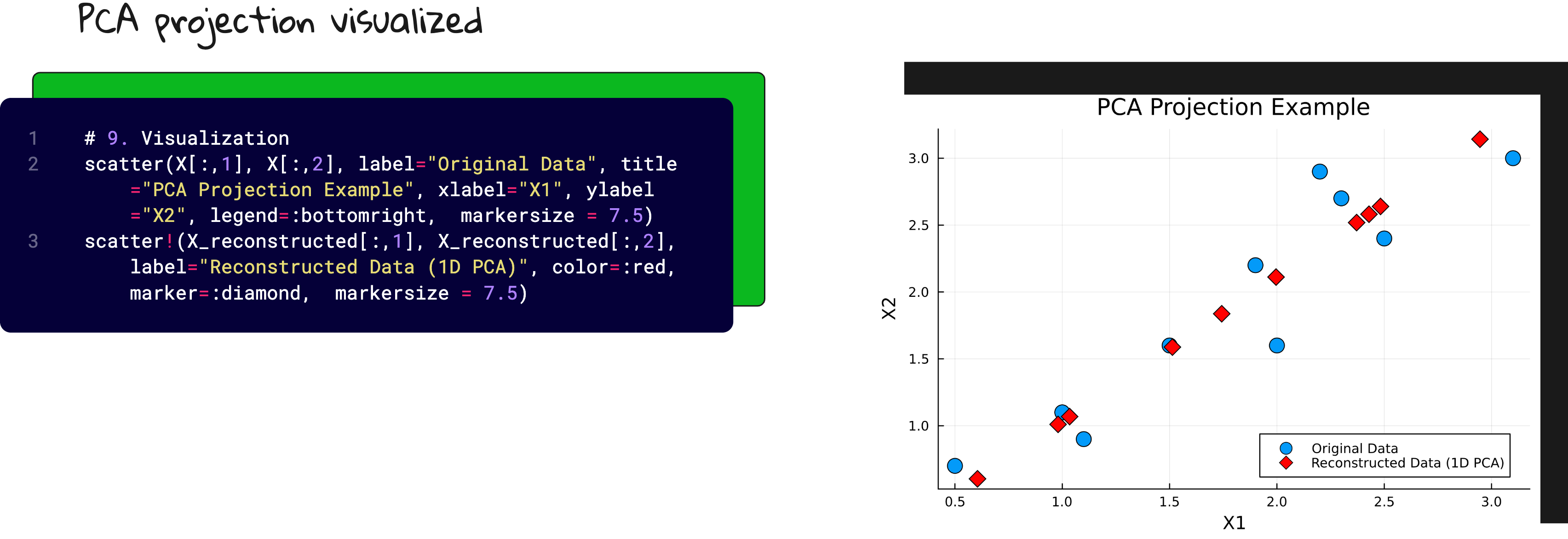
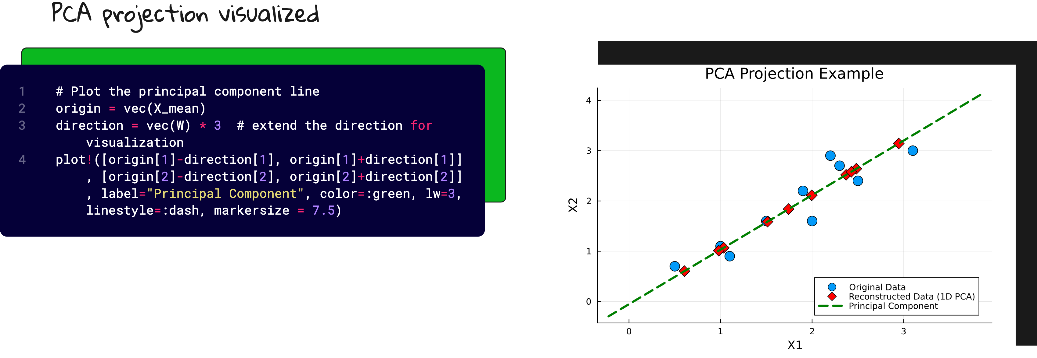
Reconstruct and visualize

And yes, I plotted the original data, the principal axis, and the projections. Because watching dots move is surprisingly satisfying when you understand what is happening.