
TurboQuant: The Surprisingly Simple Trick That's Changing How We Compress LLMs
A first-principles walkthrough of the key idea behind Google's viral quantization paper

Table of Contents:
What Is Quantization, Really?
The Outlier Problem
The Key Insight — Just Rotate It
A Concrete Example
The Second Trick — Fixing the Inner Product Bias
Why This Matters for LLM Inference
Connections and Prior Art
Every few months, a paper drops that makes the ML community collectively lose its mind. This month, it’s TurboQuant (Zandieh et al. 2025): a new vector quantization method from Google Research that achieves near-optimal compression of LLM weights and KV caches at 2.5–3.5 bits per parameter.
The Twitter discourse has been… colorful. “It’s just polar coordinates!” “It’s information theory!” “It’s magic!”
None of that is quite right. The core idea is shockingly simple, and I’m going to explain it from scratch: with visuals, concrete numbers, and zero hand-waving.
What Is Quantization, Really?
Before we get to TurboQuant, let’s make sure we’re on the same page about what quantization actually does.
You have a neural network. Every weight, every activation, every KV cache entry is a number — typically stored as a 16-bit floating point value (FP16). That’s 2 bytes per number.
A model like Llama 3 70B has 70 billion parameters. At FP16, that’s:
70B × 2 bytes = 140 GB
That doesn’t fit in a single GPU. Quantization is the art of making those numbers smaller.
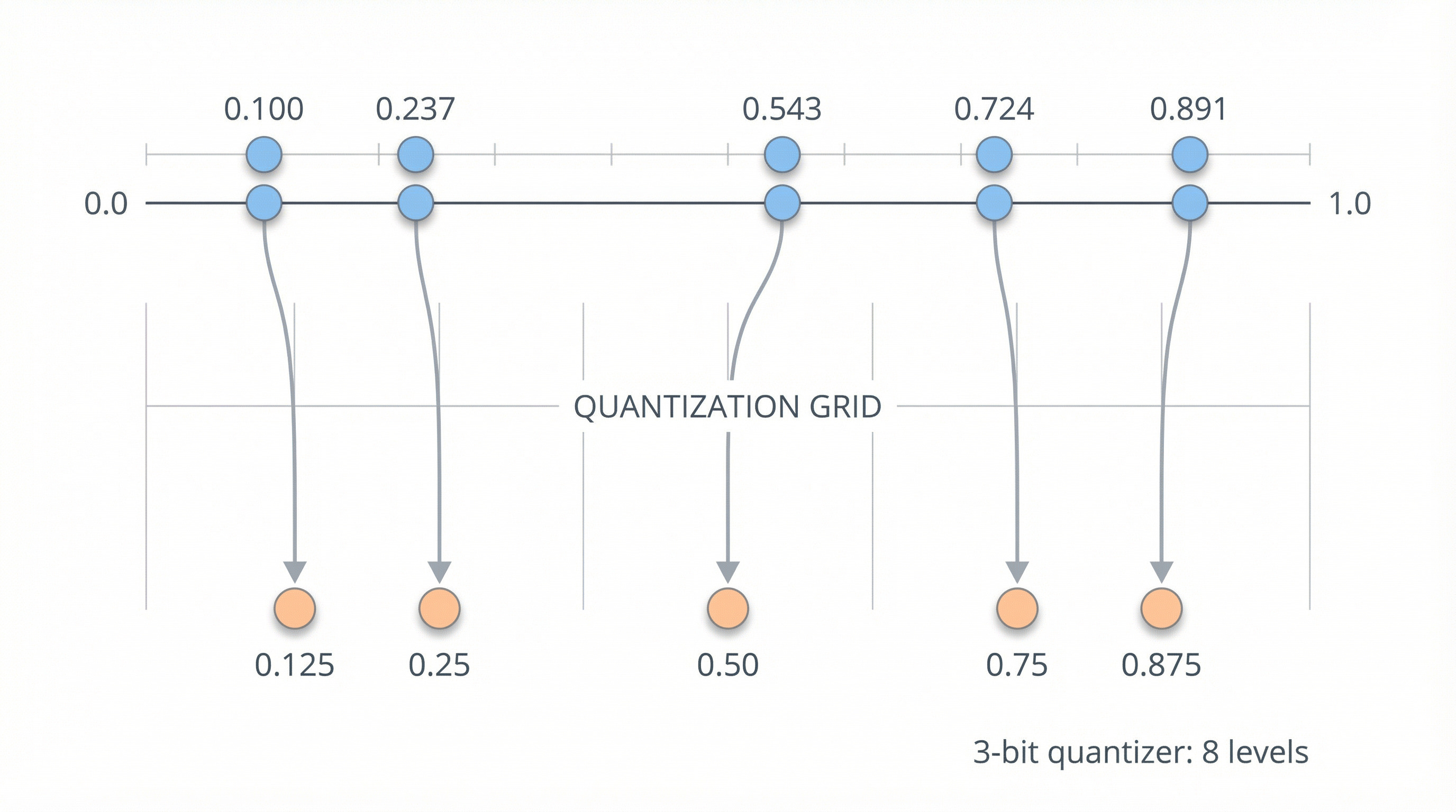
The simplest possible quantization? Just round to fewer decimal places:
Original:    0.2374623   0.7237428   0.5434738   0.1001233
Quantized:   0.237       0.724       0.543       0.100
You’ve lost some precision, but you’ve saved memory. Real quantization schemes are more sophisticated — they map continuous values to a discrete set of levels — but the core idea is always: reduce the precision of each number to use fewer bits.
At 4 bits per weight, our 70B model becomes 35 GB. At 2 bits, it’s 17.5 GB. The question is: how low can you go before the model stops working?
The Outlier Problem
Here’s where things get interesting — and where TurboQuant enters the picture.
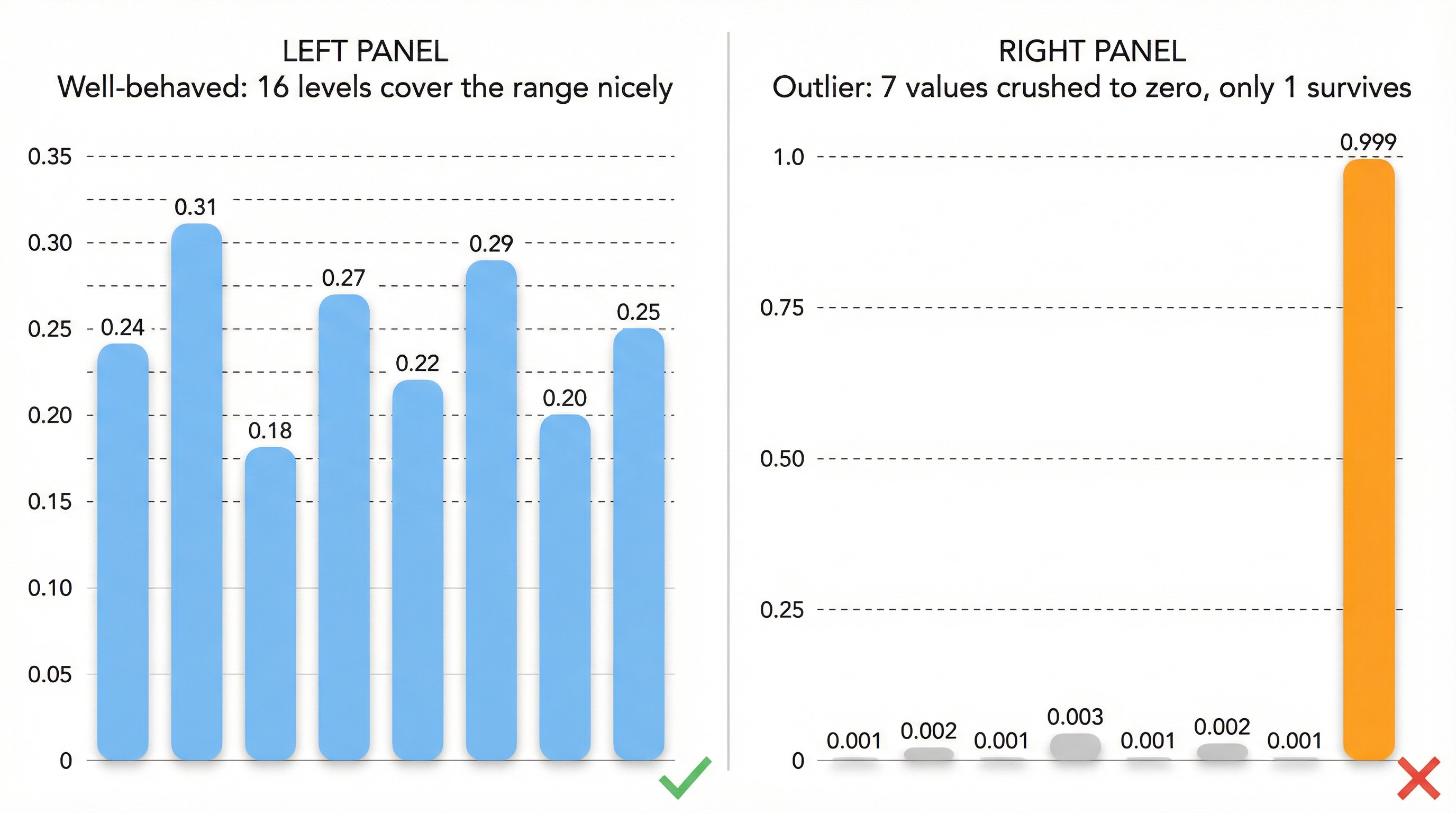
In an ideal world, the values in a neural network vector would be spread roughly evenly across their range. Something like:
Nice vector: [0.24, 0.31, 0.18, 0.27, 0.22, 0.29, 0.20, 0.25]Every component is in a similar range. If you quantize each one to 4 bits (16 levels), you can divide the range [0.18, 0.31] into 16 uniform buckets and represent each value with minimal error.
But real neural network vectors don’t look like that. They look like this:
Real vector: [0.0001, 0.9999, 0.0002, 0.0001, 0.0003, 0.0001, 0.0002, 0.0001]One component is enormous. The rest are near zero.
This phenomenon goes by many names in the transformer literature:
Whatever you call it, the effect on quantization is devastating.
Why Outliers Kill Quantization
Think about what happens when you quantize that spiky vector. Your quantization grid has to span the full range [0.0001, 0.9999]. With only 16 levels (4 bits), each bucket covers about 0.0625 of that range.
The massive component (0.9999) maps cleanly to the top bucket — no problem.
But all the tiny components (0.0001, 0.0002, 0.0003) get crushed into the very first bucket. They all become 0. The quantized vector is essentially:
Quantized: [0, 1, 0, 0, 0, 0, 0, 0]This is a cardinal direction — a unit vector pointing along a single axis. It contains almost no information. An 8-dimensional cardinal direction can be described with just log₂(2×8) = 4 bits total, but we spent 4 × 8 = 32 bits to represent it.
We’re wasting bits, and we’ve lost all the subtle information that was encoded in the small components.
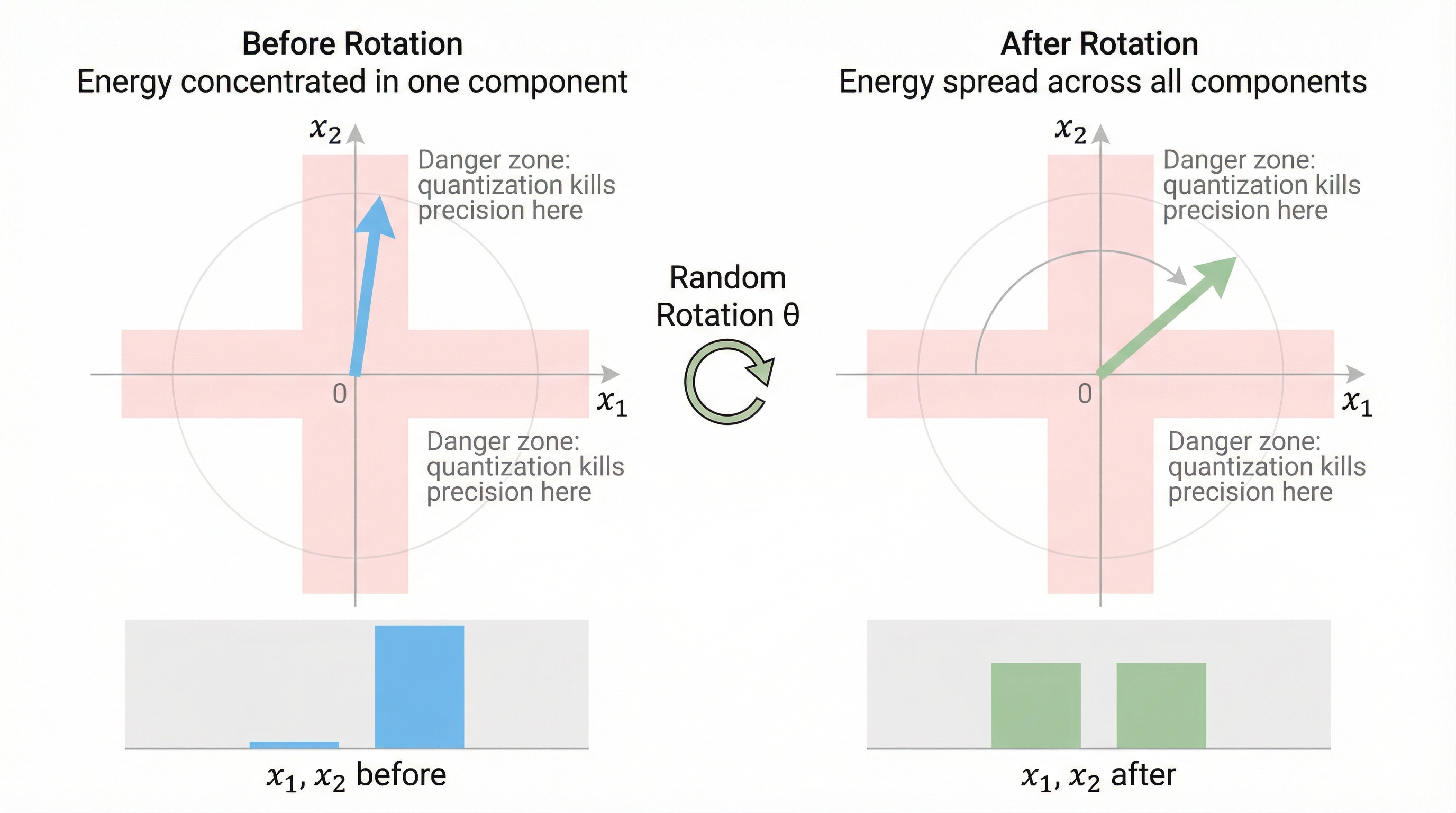
The Key Insight — Just Rotate It
Here is the entire key idea of TurboQuant, in one sentence:
Before quantizing a vector, randomly rotate it. After dequantizing, rotate it back.
That’s it. That’s the paper. (Well, most of it — there’s a clever second trick we’ll get to.)
Let me say that again, because it sounds too simple to be a major research contribution:
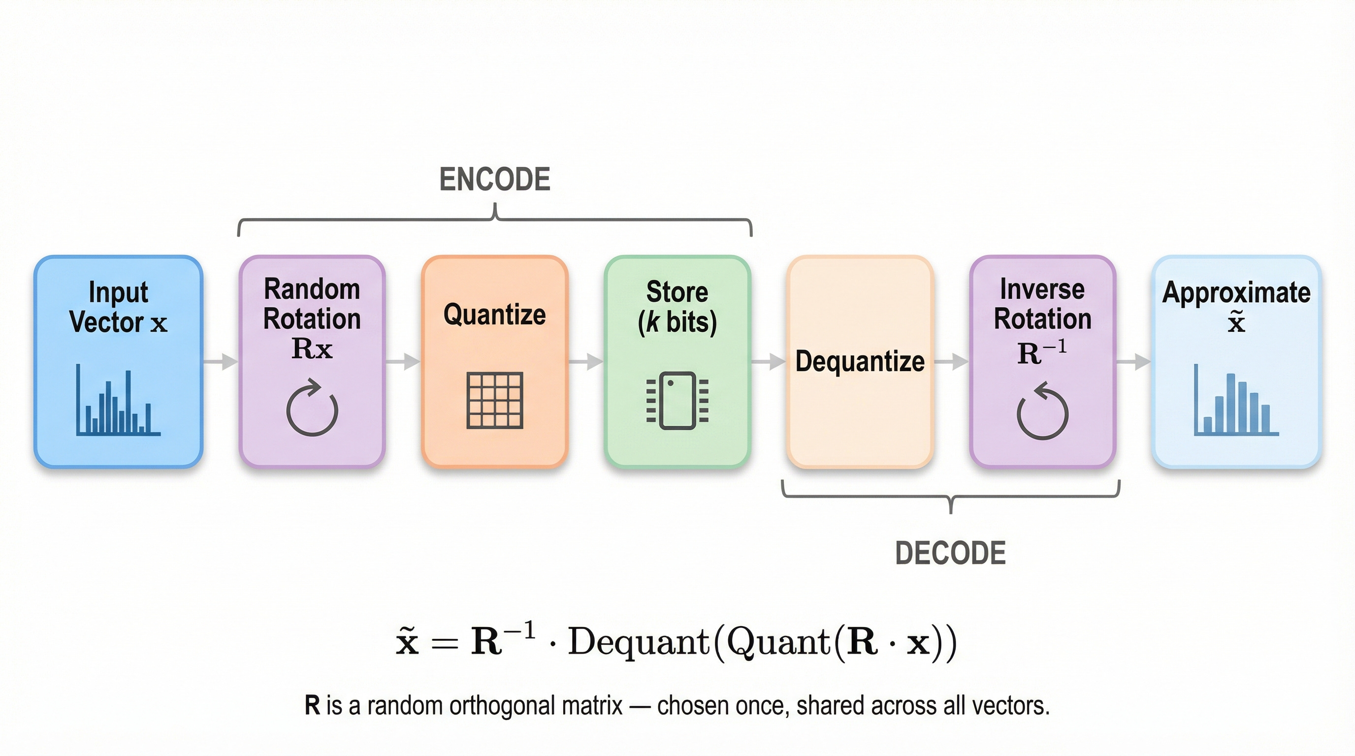
Take your vector
Multiply it by a random rotation matrix
Quantize the rotated vector
To dequantize: undo the quantization, then multiply by the inverse rotation
The rotation is data-independent. It’s chosen once and applied to everything. It doesn’t need to be learned or calibrated. It’s just a random orthogonal matrix.
But Why Does This Work?
This is the beautiful part, and it requires a little geometric intuition.
Remember our problem vector?
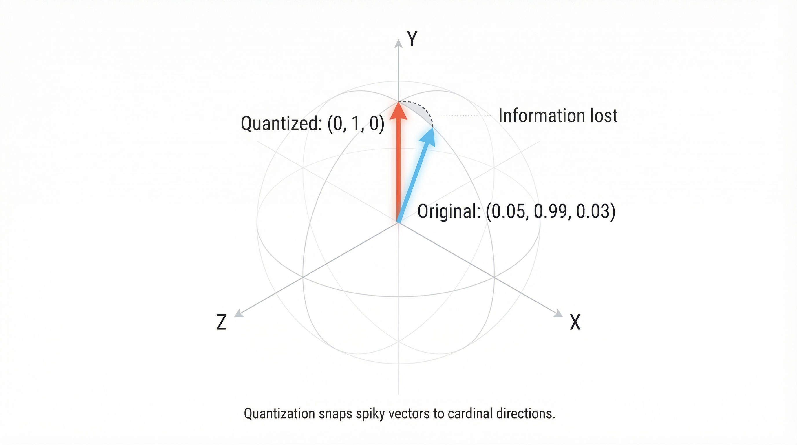
Spiky: [0.0001, 0.9999, 0.0002, 0.0001]This vector is nearly aligned with a coordinate axis — it points almost exactly in the direction of the second basis vector. Geometrically, it lives very close to one of the “poles” of the unit sphere.
Now imagine randomly rotating this vector. Where does it end up?
Almost certainly nowhere near any coordinate axis.
Think about it in 3D first. If you take a vector pointing straight up (the North Pole) and apply a random rotation, it could end up pointing in literally any direction. The chance of it landing near another pole is vanishingly small — because the poles occupy a tiny fraction of the sphere’s surface area.
After rotation, the components of our vector are spread out across all dimensions:
Before rotation: [0.0001,  0.9999,  0.0002,  0.0001]
After rotation:  [0.5012, -0.4998,  0.5001, -0.4989]
The outlier has been smeared across all components. Now each component has a similar magnitude, and our quantization grid can capture all of them with roughly equal fidelity.
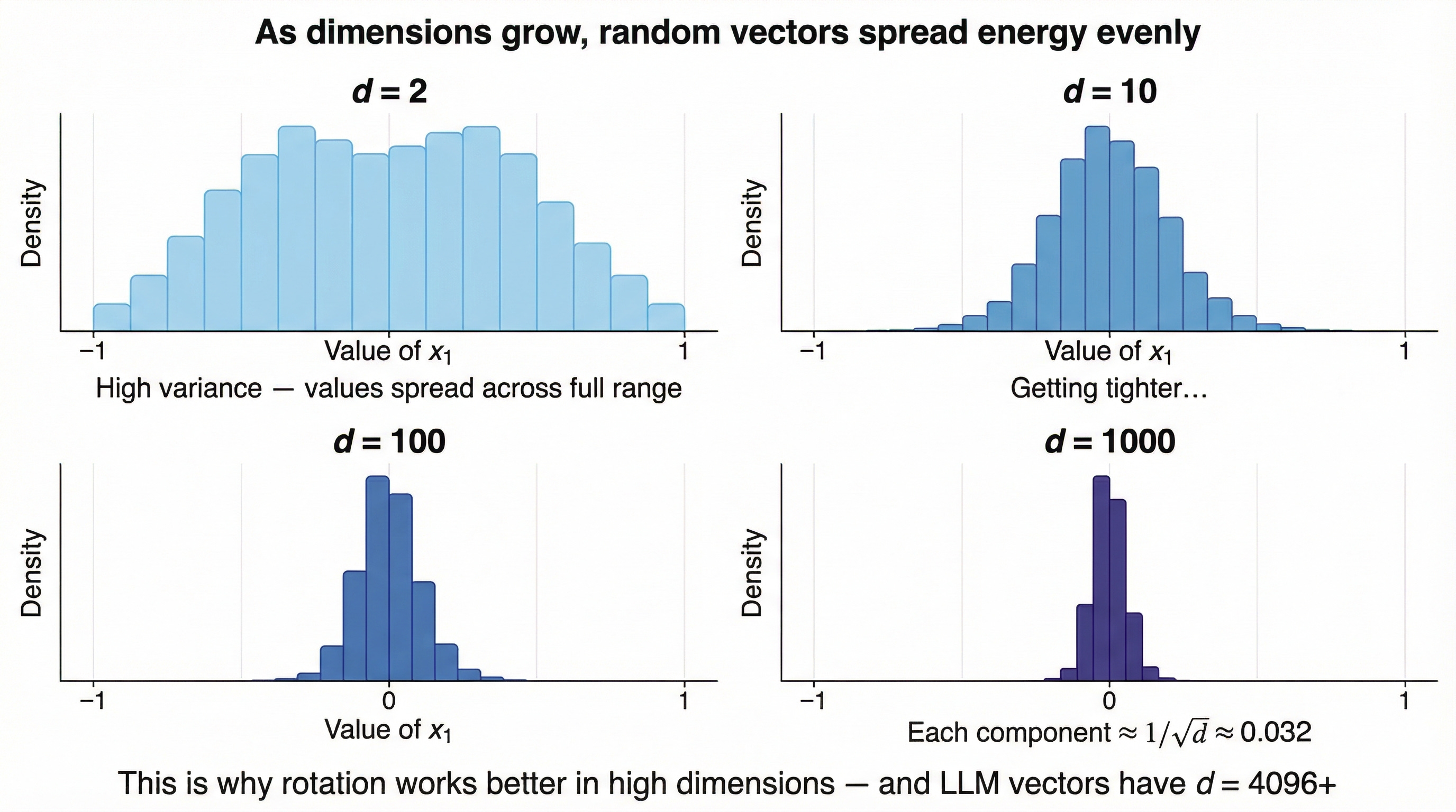
The Geometry: Why Random Directions Are “Spread Out”
Here’s the deep geometric reason this works, and it gets stronger in high dimensions.
In d dimensions, the unit sphere has a surface area that is overwhelmingly concentrated away from the coordinate axes. As d grows, the fraction of the sphere near any axis shrinks exponentially. A randomly oriented vector in high dimensions will have components that are all roughly the same size — around 1/√d each.
More precisely, after rotation, each coordinate of a unit vector follows a Beta distribution that concentrates tightly around zero. When you square each coordinate, the sum must equal 1 (because the vector has unit length), so no single coordinate can be much larger than the others.
This is a fundamental property of high-dimensional geometry, and it’s the mathematical engine behind TurboQuant.
A Concrete Example
Let’s trace through the full TurboQuant process with actual numbers. We’ll use a small 4D example.
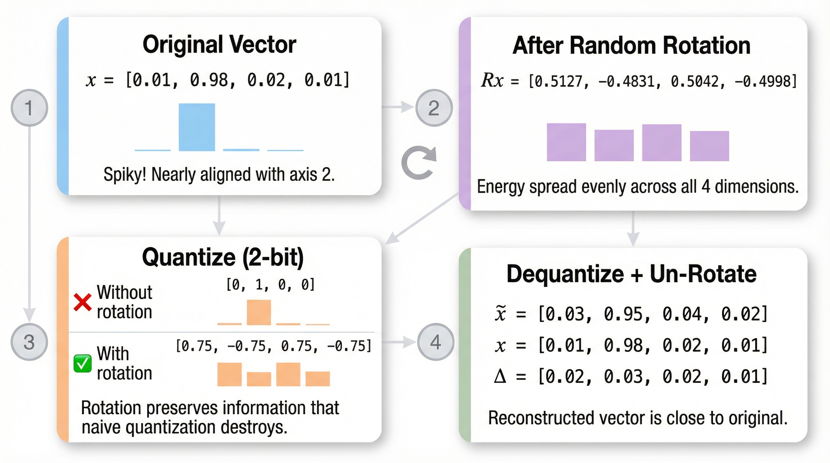
Step 1: Start With a Spiky Vector
x = [0.01, 0.98, 0.02, 0.01]Norm: ‖x‖ ≈ 0.9807
Normalized: x̂ = [0.0102, 0.9993, 0.0204, 0.0102]
Step 2: Random Rotation
We apply a random orthogonal matrix R (generated once, shared across all vectors):
x_rotated = R × x̂ = [0.5127, -0.4831, 0.5042, -0.4998]Notice: the energy is now spread evenly across all 4 dimensions. Each component has magnitude ≈ 0.5.
Step 3: Quantize
With a 2-bit quantizer (4 levels), our grid levels might be: {-0.75, -0.25, 0.25, 0.75}
x_quantized = [0.75, -0.75, 0.75, -0.75]Hmm, that’s crude — but every component gets a meaningful representation. Compare this to quantizing the original spiky vector:
Original quantized: [0.0, 1.0, 0.0, 0.0]  ← cardinal direction!
Rotated quantized:  [0.75, -0.75, 0.75, -0.75]  ← much more info!
Step 4: Dequantize and Un-Rotate
x_dequantized = R⁻¹ × x_quantized × ‖x‖
             ≈ [0.03, 0.95, 0.04, 0.02]
Compare to original: [0.01, 0.98, 0.02, 0.01]
The reconstruction is far better than the naive approach!
The Second Trick — Fixing the Inner Product Bias
TurboQuant doesn’t stop at rotation. There’s a second, more subtle insight that matters specifically for attention computation.
In a transformer’s attention layer, we don’t just store KV cache vectors — we compute inner products between queries and keys:
score = q · kIt turns out that even when rotation makes quantization better in terms of mean squared error (MSE), it can introduce a systematic bias in inner products. The quantized vectors tend to produce inner products that are slightly “off” — not randomly off, but consistently biased in one direction.
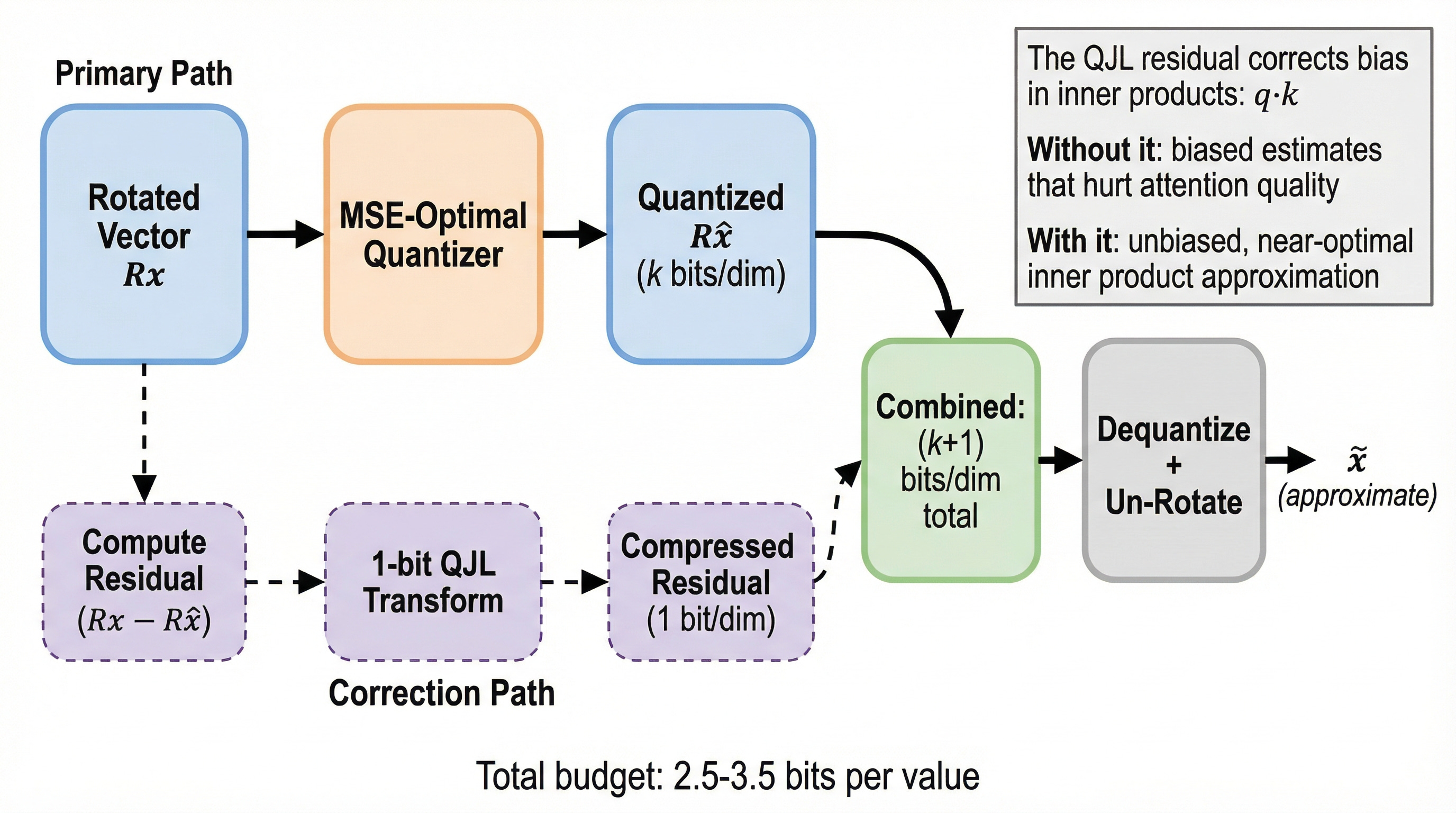
The Fix: Residual Quantization with QJL
TurboQuant uses a two-step approach:
Quantize the rotated vector using an MSE-optimal scalar quantizer (the standard part)
Compute the residual (the error between the true vector and the quantized version)
Compress the residual using a 1-bit Quantized Johnson-Lindenstrauss (QJL) transform
The QJL step takes the residual error vector and represents it with just 1 bit per dimension using a random projection. This extra bit of information is enough to correct the bias in inner product computations.
The combined system — rotation + optimal quantizer + QJL residual — achieves inner product distortion that’s within a constant factor (≈2.7×) of the information-theoretic lower bound. That’s near-optimal.
Why This Matters for LLM Inference
All of this theory is nice, but why should you care? Because TurboQuant directly addresses one of the biggest bottlenecks in LLM inference: the KV cache.
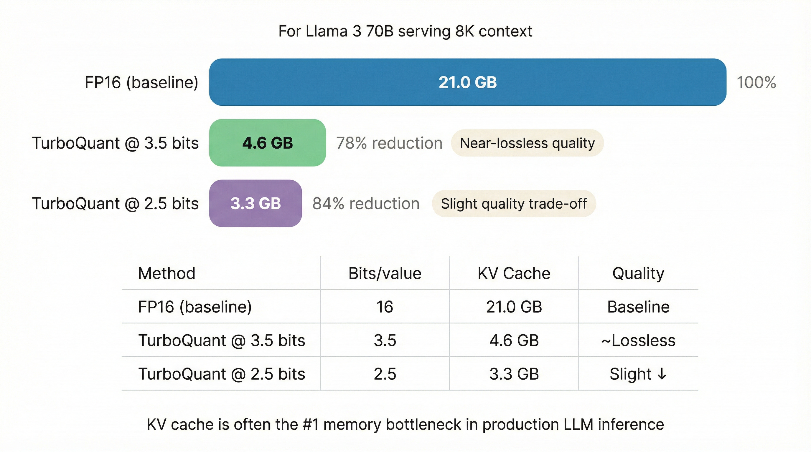
During autoregressive generation, every token you’ve processed has a key vector and a value vector stored in the KV cache. For a model like Llama 3 70B generating a sequence of 8K tokens:
KV cache = 2 (K+V) × 80 layers × 8192 tokens × 8192 dim × 2 bytes
         ≈ 21 GB
That’s 21 GB of memory just for one request’s context! For batched serving with multiple users, this quickly becomes the dominant memory cost.
TurboQuant compresses this KV cache from 16 bits to 2.5–3.5 bits per value — a 5-6× reduction — with minimal quality degradation. The paper demonstrates:
3.5 bits/value: Near-lossless quality on standard benchmarks
2.5 bits/value: Slightly degraded but still remarkably good
Training-free: No fine-tuning or calibration needed — just rotate, quantize, and go
This is what makes TurboQuant so exciting for production inference. It’s simple to implement, requires no retraining, and achieves near-optimal compression.
Connections and Prior Art
TurboQuant isn’t the first method to use rotation for quantization. Two notable predecessors:
QuIP (Chee et al. 2023) uses random orthogonal transformations for weight quantization, with a similar intuition about spreading outlier energy. However, QuIP uses the rotation as part of a more complex optimization procedure, while TurboQuant isolates the rotation as a standalone preprocessing step with clean theoretical guarantees.
RaBitQ (Gao et al. 2024) employs random rotation for vector database compression and nearest-neighbor search. TurboQuant extends this idea with the bias-correcting QJL step, which is critical for the inner product computations in attention.
What TurboQuant contributes beyond these is: (1) a clean theoretical analysis showing the rotation + quantizer is near-optimal, (2) the bias correction via QJL for inner products, and (3) a practical demonstration on LLM KV cache compression.
The Takeaway
Neural network vectors tend to be “spiky” — nearly aligned with coordinate axes. Quantization snaps spiky vectors to cardinal directions, destroying information. A random rotation spreads the energy evenly across all dimensions, making every component equally important and equally well-served by the quantization grid.
The fix is almost embarrassingly simple: multiply by a random rotation matrix before quantizing, and multiply by its inverse after dequantizing. No training. No calibration. No data dependence. Just linear algebra.
Combined with a 1-bit residual correction for inner product bias, this yields a quantization scheme that’s within a small constant factor of the information-theoretic limit.
Sometimes the most impactful ideas in ML aren’t the most complex ones. They’re the ones that see a fundamental geometric truth that was hiding in plain sight.