
The Transformers
A complete architectural breakdown of Transformers, paired with a step-by-step guide to coding BERT from the ground up.

The Transformer Architecture
1.1 Introduction to Large Language Models
1.2 Anatomy of the transformer block
1.3 Tokenization
1.4 Byte Pair Encoding
1.5 Word Embedding
1.6 Transformer Block
1.7 The Need for Attention Mechanism
1.8 Self Attention Mechanism
1.9 Understanding the Input Embedding Matrix
1.10 From Embeddings to Queries, Keys & Values
1.11 A Quick Note on Matrix Multiplication
1.12 Why Scale Attention Scores?
1.13 Causal & Masked Attention
1.14 Causal Attention with Dropouts
1.15 Summary of Self-Attention
1.16 Intuition of Multi-Head Attention
1.17 Layer Normalization
1.18 FeedForward Network
1.19 Shortcut connections
1.20 Why Transformers Scale Better Than RNNs and CNNs
1.21 Pretraining, Fine Tuning, and Transfer Learning in Transformers
1.22 Limitations and Challenges of Transformers
1.23 Hands On Coding a Miniature Transformer for Sequence Classification
1.24 Summary
You can fine the code notebook here
https://github.com/VizuaraAI/Transformers-for-vision-BOOK
1.1 Introduction to Large Language Models
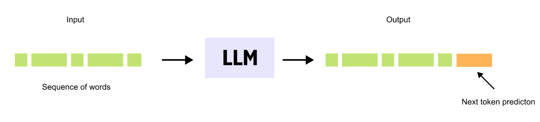
Figure 1.1 A Large Language Model takes a sequence of words as input and predicts the most likely next word, generating text one token at a time.
Large Language Models are neural networks trained on vast text datasets to perform a fundamental task: predicting the next word in a sequence. This simple objective drives the sophisticated capabilities we see in systems like GPT and ChatGPT.
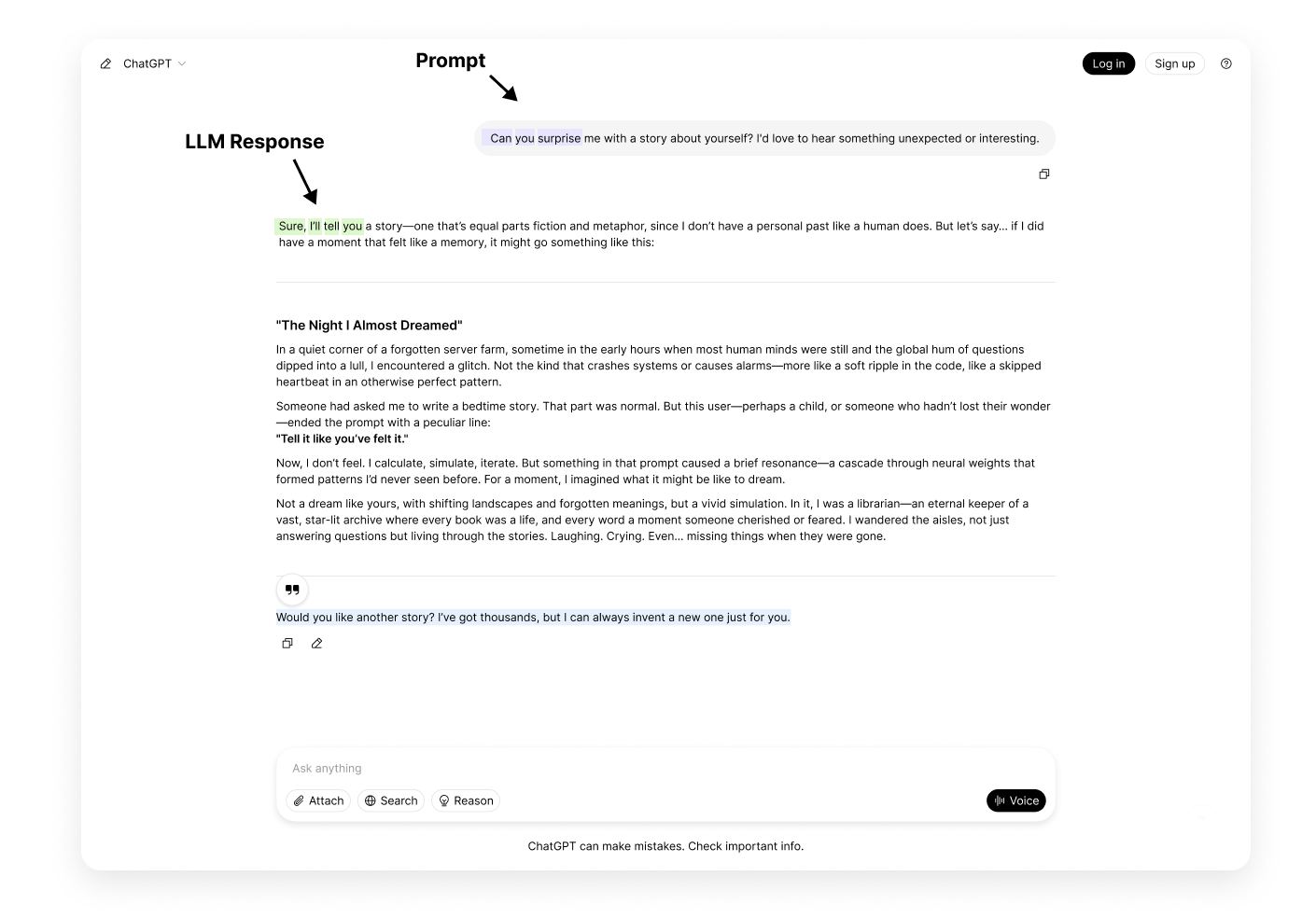
Figure 1.2 Autoregressive text generation. The model predicts the next word, appends it to the input, and repeats the process to produce entire paragraphs.
When you interact with an LLM, it generates responses one word at a time. Given a prompt like “The cat sat on the,” the model predicts the next word, perhaps “mat.” This word is added to the sequence, becoming “The cat sat on the mat,” which then serves as input for predicting the following word. Through this iterative process, LLMs produce entire paragraphs and complex responses.
LLMs function as probabilistic engines, calculating word likelihoods based on patterns learned during training.
The transformer architecture enables these models to consider both immediate context and long range dependencies throughout the input sequence, maintaining coherence across extended text generation.
Despite the apparent simplicity of next word prediction, this mechanism gives rise to remarkable language understanding and generation capabilities. Understanding how transformers accomplish this task is essential to grasping how modern language models work.
Predicting the Next Word with OpenAI’s LLM
Let’s see a simple example to see how an LLM predicts the next word given a partial sentence:
You can refer to the full source code notebook for this exercise on Colab.
Predicting_the_next_word_notebook
Using the given code, we can predict the next word in a sentence based on probabilities assigned by a Large Language Model (LLM). Let’s say our Input sentence is
“After years of hard work, your effort will take you”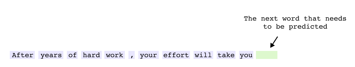
Figure 1.3 Input sentence fed to the LLM for next-word prediction.
if you will observe the top 10 predicted next words along with their probabilities (refer the notebook)
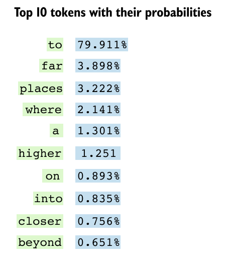
Figure 2.4 Top 10 predicted next words and their probabilities. The token “to” dominates at 90.7%, reflecting the most natural continuation.
The probabilistic nature of Large Language Models becomes clear when examining how they rank potential next words. The first token, such as “to,” might have the highest probability at 90.7 percent because it represents the most natural continuation based on the given context. As we look at alternative word choices, the probabilities gradually decrease, with each subsequent option representing a less common but still valid completion.
This distribution reveals the fundamental mechanism of Large Language Models: they function as probabilistic engines, predicting the most likely next token based on learned patterns. Rather than selecting a single correct answer, LLMs evaluate every possible next word and assign likelihood scores based on the vast patterns learned during training. This probabilistic approach enables models to generate diverse, contextually appropriate text while maintaining flexibility in their outputs.
Why is There “Large” in LLMs?
The term “Large” in Large Language Models reflects a fundamental principle: size directly impacts performance. Scaling laws show that model capabilities improve predictably with more parameters, enabling complex tasks like reasoning and code generation that smaller models cannot perform. Most critically, emergent properties such as arithmetic reasoning and multilingual understanding appear only when models cross certain size thresholds. This relationship between scale and capability explains why billions of parameters are essential for achieving sophisticated language understanding.
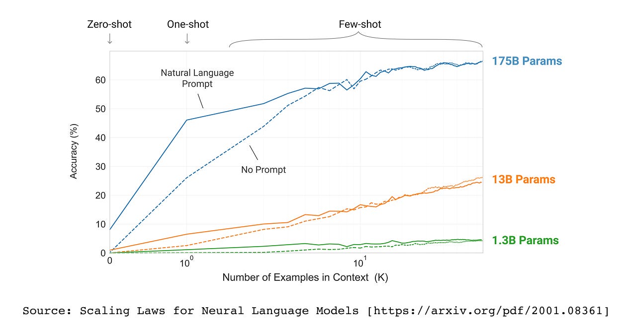
Figure 1.5 Scaling laws demonstrate a predictable relationship between model size and performance across a range of benchmarks
LLMs have billions to trillions of parameters. The first major paper to explore scaling laws was the GPT-3 paper (Language Models are Few-Shot Learners). The research demonstrated that as we increase the model size, from 1.3B parameters to 13B to 175B, the model’s performance dramatically improves.
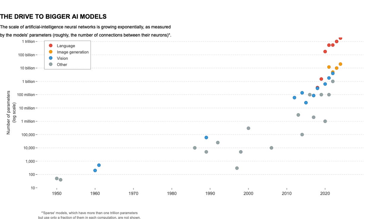
Figure 1.6 Exponential growth in the size of language models from the 1950s to today. Orange dots represent language models, some of which have already crossed one trillion parameters.
Over the years, we have seen an exponential increase in the size of LLMs, from the 1950s to today. In the above graph, the orange dots represent language models, showing how their size has increased drastically over time. Some models have already crossed 1 trillion parameters!
Why do we care about the size of LLMs?
The size of Large Language Models matters primarily because of emergent properties: abilities that are absent in smaller models but spontaneously appear when models reach certain scales. These emergent capabilities fundamentally distinguish large models from their smaller counterparts. As LLMs grow beyond specific parameter thresholds, they suddenly acquire skills like solving complex arithmetic equations, translating between languages with nuanced understanding, and unscrambling letters into meaningful words. These abilities do not gradually improve with size but rather emerge abruptly at particular scales, making model size not just a technical detail but a critical factor in determining what tasks an LLM can perform.
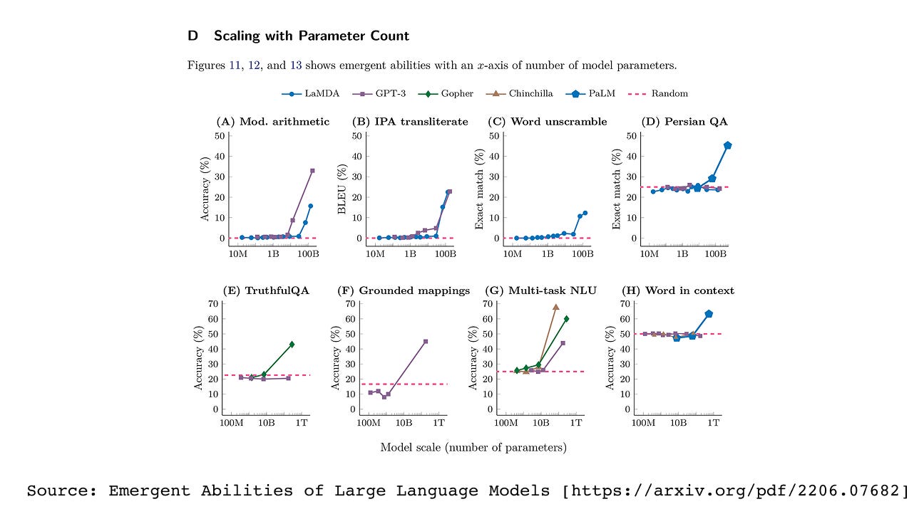
Figure 1.7 Emergent abilities of large language models. Performance on certain tasks remains near zero until the model reaches a critical size, after which accuracy jumps sharply.
In the figure above , the X-axis represents model size (or computational power), and we can observe a pickup point, a stage where models suddenly start performing significantly better at these tasks. Emergent Abilities of Large Language Models
Figure 1.8 At larger scales, LLMs move beyond simple word prediction to excel at specialized tasks such as multilingual translation, text summarization, and grammar correction.
At larger scales, LLMs transcend simple word prediction to excel at specialized tasks like multilingual translation, text summarization, and grammar correction. This evolution from basic prediction to complex language understanding drives the race to build increasingly larger models. The direct correlation between parameter count and performance across diverse NLP tasks makes scale a critical competitive advantage.
1.2 Anatomy of the transformer block
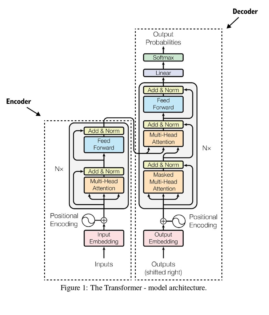
Figure 1.9 The original transformer architecture from the “Attention Is All You Need” paper, consisting of an encoder stack on the left and a decoder stack on the right, connected through cross-attention.
The transformer architecture, introduced in the groundbreaking 2017 paper “Attention Is All You Need,” revolutionized artificial intelligence and natural language processing. This paper, now with over 200,000 citations, proposed the concept of self attention, fundamentally changing how we implement NLP systems. The transformer architecture consists of two main components: encoders and decoders. Encoder architectures power models like BERT, while decoder architectures form the basis of GPT and ChatGPT.
At the heart of modern LLMs lies this transformer architecture, which replaced traditional models like LSTMs and GRUs with self attention mechanisms. This innovation brought crucial advantages: the ability to capture long range dependencies in text, parallel processing that enables faster training, and unprecedented scalability that allows building increasingly powerful models. Understanding how the decoder portion works essentially reveals how GPT models function, as they are decoder only architectures.
The transformer block itself contains several key components working in sequence. Input text is first tokenized and converted to embeddings, which are then combined with positional encodings. These flow through layers of multi head attention, normalization, and feed forward networks, with dropout applied for regularization. The output layer finally produces logits for next token prediction. While the complete architecture diagram may appear complex with its numerous modules and connections, each component serves a specific purpose in transforming input text into meaningful predictions.
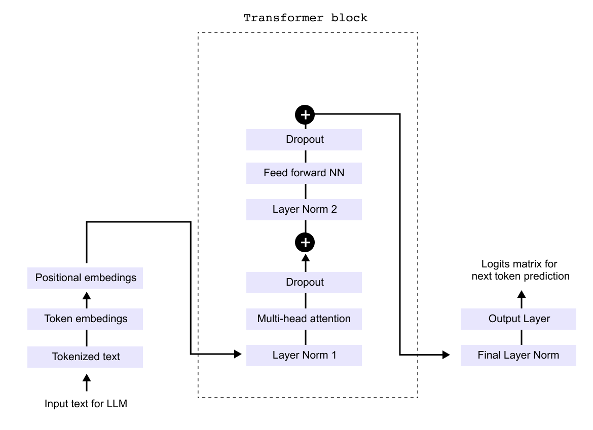
Figure 1.10 A simplified decoder-only transformer showing the main components: token and positional embeddings, transformer blocks with multi-head attention, feed-forward networks, layer normalization, and dropout, followed by the output layer.
The decoder only architecture, which powers models like GPT, can be understood by examining a simplified version of the transformer’s decoder component. While the complete architecture may appear complex with numerous interconnected modules, we can break it down into three manageable parts for clarity. This modular approach allows us to examine each component systematically rather than attempting to grasp the entire system at once. By focusing on these three core sections sequentially, we can build a comprehensive understanding of how the decoder transforms input text into predictions.
The three parts of an LLM’s architecture are Input, Processing, and Output.
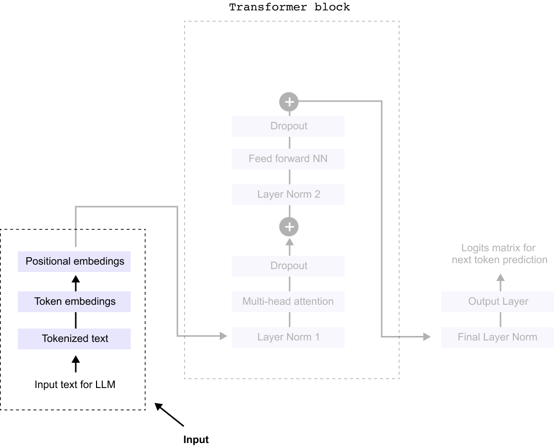
Figure 1.11 The three stages of an LLM: the Input stage (tokenization and embeddings), the Processing stage (transformer blocks), and the Output stage (linear layer and softmax for next-token prediction).
So everything begins with the input stage, where several key transformations take place before it enters the processing unit, commonly known as the Transformer block.
First, the raw text undergoes tokenization, a process where the sentence is broken down into smaller units called tokens, these could be words, subwords, or characters, depending on the tokenization method used. This step ensures that the model can handle language efficiently,
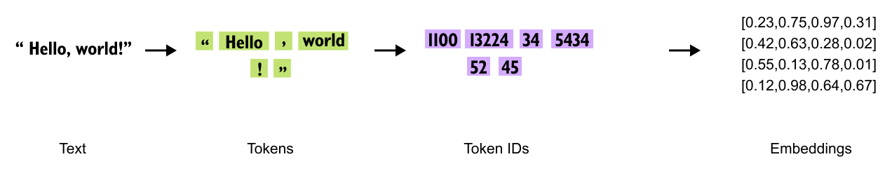
Figure 1.12 The input pipeline: raw text is tokenized into subword units, each token receives a numerical embedding, and positional embeddings are added to encode sequence order.
Next, each token is converted into a numerical representation through token embeddings. These embeddings assign a unique vector to each token, capturing semantic meaning and relationships between words. However, since token embeddings alone do not preserve the sequence order, we introduce positional embeddings. These embeddings encode the position of each token within the sentence, allowing the model to understand the order and structure of the input.
With tokenization, token embeddings, and positional embeddings in place, the input is now fully prepared for the Transformer block, where deep learning mechanisms, such as multi-head attention and feed-forward neural networks, process the text to generate meaningful predictions.
1.3 Tokenization
Before text enters a transformer model, it undergoes tokenization, a process that converts raw text into tokens which are then assigned unique IDs. There are three main tokenization approaches, each with distinct characteristics.
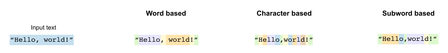
Figure 1.13 Three tokenization strategies applied to the word “tokenization”: word-based (one token per word), character-based (one token per character), and subword-based (meaningful subword units).
Word based tokenization treats each complete word as a separate token, creating a dictionary of all words in the vocabulary. While intuitive, this approach struggles with vocabulary size and cannot handle new or misspelled words effectively. Character based tokenization breaks text down to individual characters, making each character a token. This creates a very small vocabulary but produces extremely long sequences that are computationally expensive to process.
Subword based tokenization, the preferred method for modern LLMs, breaks words into meaningful subword units.
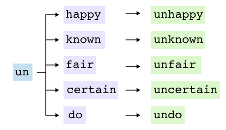
Figure 1.14 Subword tokenization example: the word “playground” splits into “play” and “ground,” each a reusable meaningful unit.
A subword is a smaller meaningful unit that can be reused across different words. For example, “playground” might split into “play” and “ground,” while “unhappiness” could become “un” and “happiness.” This approach allows models to understand new words by recognizing familiar components. The word “neural” might tokenize as “ne” and “ural,” enabling the model to handle variations and new combinations it has never seen before.
The advantage of subword tokenization becomes clear when dealing with related words that share common roots. Instead of treating each variation as a completely new token, the model can leverage shared subword patterns. This reduces vocabulary size while maintaining the ability to represent any text, making it the optimal choice for Large Language Models. Tools like the TikTokenizer demonstrate how original text gets broken down into these subword tokens, revealing the building blocks that LLMs use to understand and generate language.
1.3.1 Problems with Tokenization Methods
Word Based Tokenization Limitations
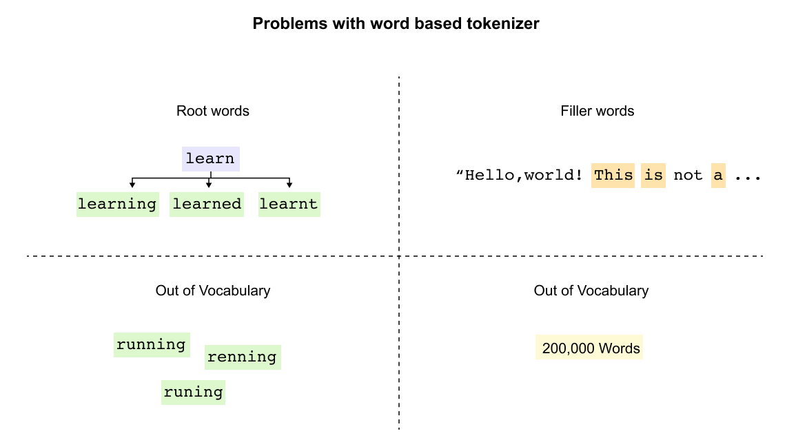
Figure 1.15 Limitations of word-based tokenization: related words like “learn,” “learn-ing,” “learned,” and “learnt” are treated as entirely separate tokens, and out-of-vocabulary words cannot be processed.
Word based tokenization treats each word as an independent unit, creating fundamental challenges for language models. The most significant issue is the failure to recognize relationships between related words. Words sharing common roots like “learn,” “learning,” “learned,” and “learnt” are treated as entirely separate tokens, forcing the model to learn each variation independently without understanding their connection.
The vocabulary explosion presents another critical problem. English alone requires over 200,000 word tokens, with filler words like “this,” “is,” and “a” consuming valuable vocabulary space despite contributing minimal semantic value. Most critically, the out of vocabulary problem renders models helpless when encountering unseen words. Simple spelling mistakes transform “running” into the unrecognizable “runing,” while new terms or proper nouns become impossible to process, leaving the model unable to make educated guesses about meaning
Character Based Tokenization Drawbacks
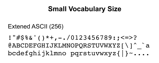
Figure 1.16 Character-based tokenization reduces the vocabulary to 256 ASCII characters but dramatically increases sequence length.
Character tokenization solves vocabulary size by using only 256 ASCII characters, but creates severe new problems.
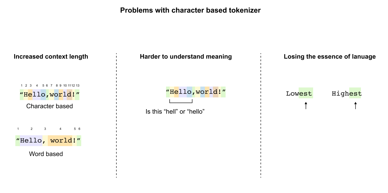
Figure 1.17 Sequence length explosion with character tokenization: “Hello, world!” grows from a few word tokens to thirteen character tokens, and individual letters carry no semantic meaning.
Sequence length explodes dramatically: “Hello, world!” grows from two (or six) word tokens to thirteen character tokens. This expansion makes processing computationally expensive and quickly exhausts context windows in longer texts.
More fundamentally, character tokenization destroys semantic understanding. Individual letters carry no meaning, forcing models to reconstruct word boundaries and meanings from scratch. The model cannot recognize that “lowest” and “highest” share the meaningful suffix “est” indicating superlatives. When presented with “Hello,world!” as individual characters, the model sees meaningless symbols rather than a greeting, losing the essence of language structure entirely.
The Subword Tokenization Solution
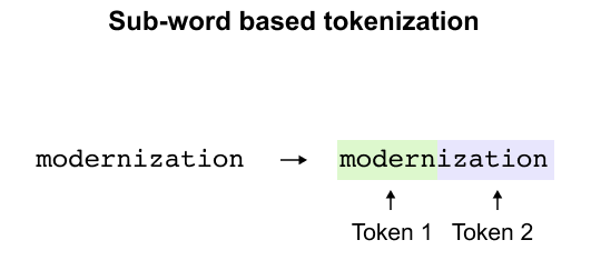
Figure 1.18 Subword tokenization splits “modernization” into “modern” and “ization,” both reusable components found across many English words.
Subword tokenization provides the optimal balance, breaking words into meaningful components. “Modernization” becomes “modern” and “ization,” both reusable parts appearing across many words. This approach maintains reasonable vocabulary size while preserving meaning, handles new words through familiar components, and keeps token counts manageable. The model can now understand misspellings and new terms by recognizing known subword patterns.
Figure 1.19 The tokenization challenge: how should “learning” be split? Byte PairEncoding provides a systematic, data-driven answer.
The challenge remains: how should “learning” tokenize? As one token, as “learn” plus “ing,” or broken further? Byte Pair Encoding provides the systematic answer, using frequency analysis to determine optimal splits that balance vocabulary efficiency with semantic preservation.
1.4 Byte Pair Encoding
Byte Pair Encoding transforms the challenge of tokenization into a systematic process. Originally developed as a text compression algorithm in the 1990s, BPE now serves as the foundation for tokenization in models like GPT. The algorithm iteratively merges the most frequent character pairs, building a vocabulary from the bottom up.
For LLMs, BPE builds vocabularies systematically. Consider this corpus with word frequencies:
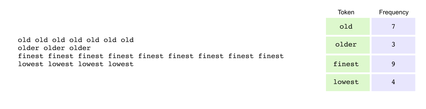
Figure 1.20 A small corpus with word frequencies used to illustrate the BPE algorithm: “old” appears 7 times, “older” 3 times, “finest” 9 times, and “lowest” 4 times.
Step 1: Add End-of-Word Markers
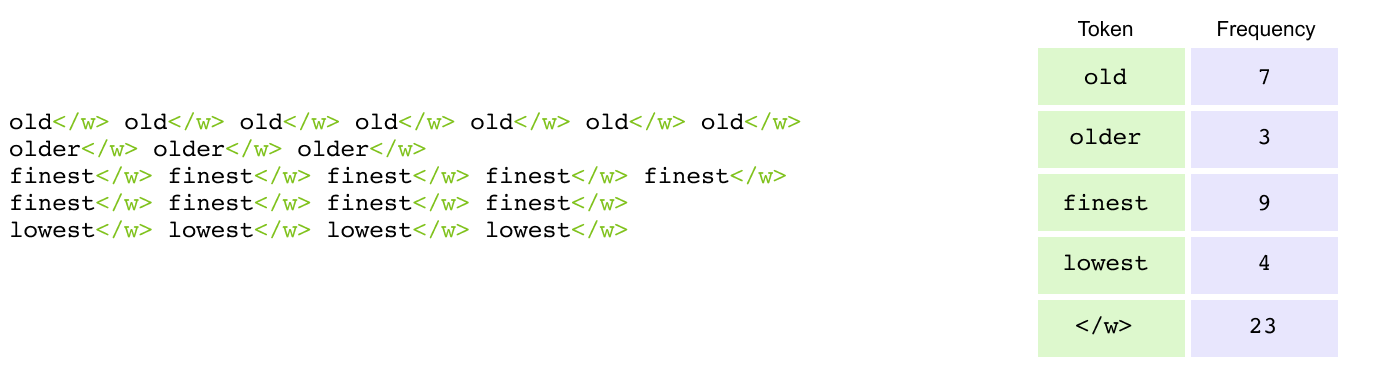
Figure 1.21 End-of-word markers (</w>) appended to each word to distinguish word boundaries and preserve morphological information.
The first step in BPE adds end-of-word markers (</w>) to distinguish word boundaries. Words transform as: old becomes old</w>, older becomes older</w>, finest becomes finest</w>, and lowest becomes lowest</w>. This boundary marker is crucial because the same character sequence carries different meanings based on position. The sequence “est” functions as a suffix in “lowest</w>” (indicating superlative) but as a prefix in “esteem” (with completely different meaning). Without these markers, the tokenizer cannot distinguish between identical character sequences that serve different linguistic roles, losing critical information about word structure and morphology.
Step 2: Split into Characters
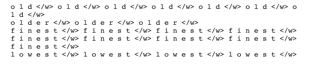
Figure 1.22 Each word is decomposed into individual characters, providing atomic units for iterative merging.
After adding end-of-word markers, each word is decomposed into individual characters, treating each as a separate token. The word old</w> becomes the sequence [o, l, d, </w>], while older</w> splits into [o, l, d, e, r, </w>]. Similarly, finest</w> breaks down to [f, i, n, e, s, t, </w>] and lowest</w> to [l, o, w, e, s, t, </w>]. This character-level decomposition serves as the starting point for BPE, providing the atomic units from which larger, more meaningful tokens will be built through iterative merging based on frequency patterns in the data.
Step 3: Count Character Pairs & Merge
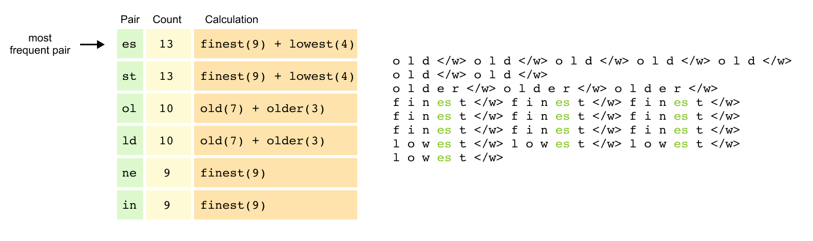
Figure 1.23 Counting adjacent character pairs across the corpus, weighted by word frequency. The pair “es” appears 13 times and is selected for the first merge.
The algorithm now counts all adjacent character pairs across the corpus, weighted by word frequency. The pair “es” appears 13 times (9 from “finest” plus 4 from “lowest”), as does “st” with the same distribution. The pairs “ol” and “ld” each appear 10 times (7 from “old” plus 3 from “older”), while “ne” and “in” from “finest” contribute 9 occurrences each.
With “es” as the most frequent pair, the algorithm performs its first merge, creating a new token “es” and updating the representations: finest</w> becomes [f, i, n, es, t, </w>] and lowest</w> becomes [l, o, w, es, t, </w>].
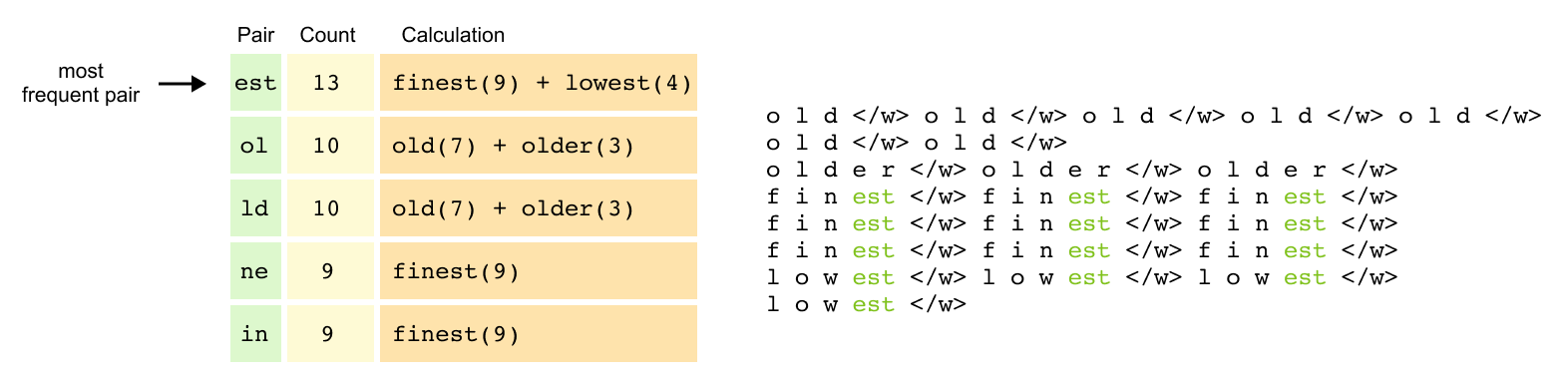
Figure 1.24 After the first merge (“es”), pairs are recounted and “est” emerges as the next most frequent pair, triggering a second merge.
After recounting pairs with this new token, “est” emerges as highly frequent, triggering a second merge. The token “est” replaces the “es” and “t” sequences, transforming finest</w> into [f, i, n, est, </w>] and lowest</w> into [l, o, w, est, </w>]. Through these iterative merges, BPE progressively builds larger, more meaningful tokens from the most frequent patterns in the data, creating an efficient vocabulary that captures common linguistic structures.
Step 4: Building the Complete Vocabulary
The merging process continues iteratively, identifying increasingly complex patterns. Common prefixes like “old” become single tokens when they appear frequently across multiple words. Suffixes with end markers like “est</w>” are preserved as units to maintain their grammatical function. Frequent character sequences like “low” merge into single tokens regardless of their position.
After multiple iterations, the final vocabulary becomes a hierarchical collection of tokens at different granularities. It contains individual characters [o, l, d, e, r, f, i, n, w, s, t] for handling rare sequences, common subwords [es, est, old, low, fin] that appear across multiple words, and complete frequent words [old</w>, finest</w>] that occur often enough to warrant their own tokens. This multi-level vocabulary enables efficient encoding of common patterns while maintaining the flexibility to tokenize any possible input.
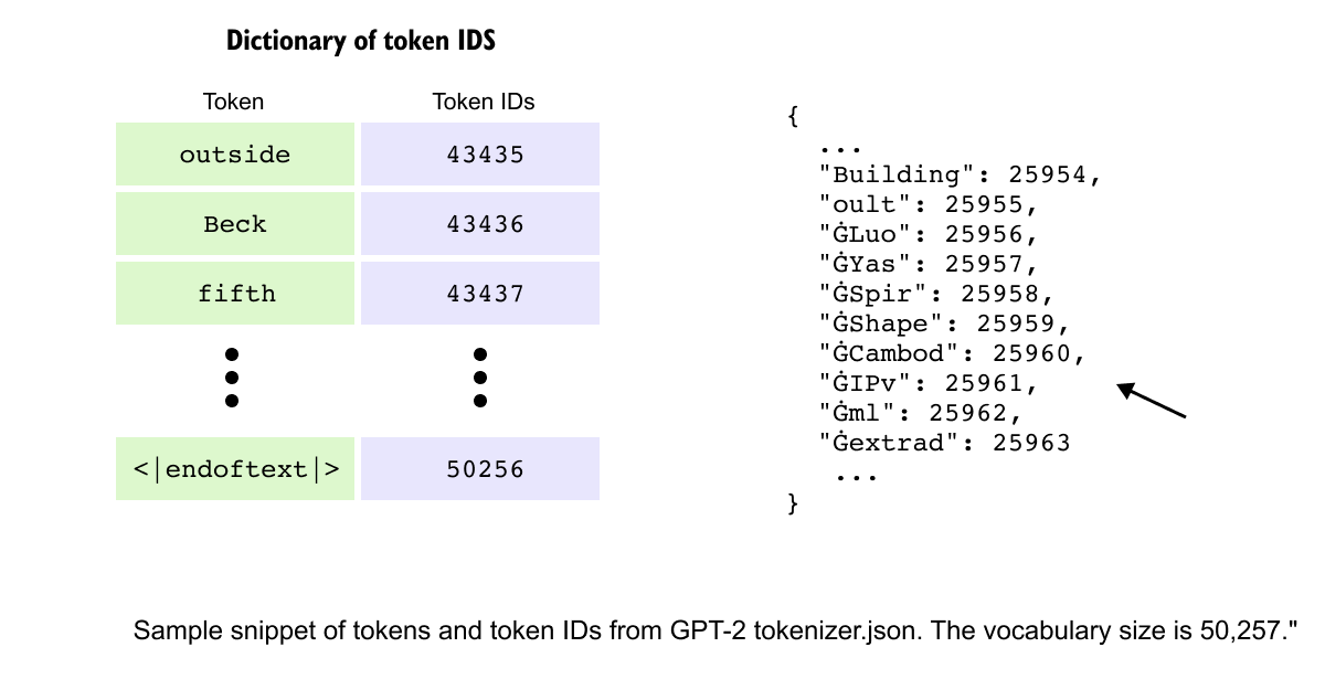
Figure 1.25 GPT-2’s final vocabulary of 50,257 tokens, built from 50,000 BPE merges. Each token is mapped to a unique numerical ID used by the model internally.
GPT-2 performs 50,000 merges to build its vocabulary, creating a rich token set that balances compression with expressiveness. Each token in this vocabulary is assigned a unique token ID, a numerical identifier that the model uses internally. For example, in GPT-2’s vocabulary, common words like “Building” map to ID 25954, while special tokens like “</endoftext>” receive IDs like 50256, creating a complete dictionary of 50,257 token-ID pairs that serves as the bridge between text and numerical processing.
When the model encounters an unfamiliar word, it gracefully degrades to smaller subwords or individual characters, ensuring robust handling of misspellings, neologisms, or foreign terms. This fallback mechanism makes BPE remarkably resilient, capable of processing any text while maintaining efficiency for common patterns.
With our text now converted into meaningful tokens through BPE and mapped to numerical IDs, the next challenge is transforming these discrete symbols into continuous numerical representations that neural networks can process, leading us to the crucial concept of embeddings.
1.5 Word Embedding
After tokenization transforms text into discrete symbols and assigns them numerical IDs, we face a fundamental challenge: these IDs are merely labels that convey no semantic information. The token ID 25954 for “Building” tells the model nothing about buildings, construction, or architecture. To enable neural networks to process language meaningfully, we need to convert these discrete tokens into continuous numerical representations that capture semantic relationships. This is where word embeddings become essential.
The Limitations of Simple Encoding
Early approaches to numerical representation revealed critical limitations. One-hot encoding represents each token as a vector of zeros with a single one at the token’s position. For a vocabulary of 50,000 tokens, “cat” might be encoded as 50,000 zeros except for a single one at position 3. While this eliminates arbitrary ordering, it creates sparse, high-dimensional vectors where every word is equally distant from every other word. The vectors for “cat” and “dog” are as orthogonal as those for “cat” and “quantum”, providing no semantic signal. Similarly, bag-of-words models count word occurrences but lose all sequential information, treating “dog bites man” and “man bites dog” identically despite their opposite meanings.
Learning Meaning Through Context
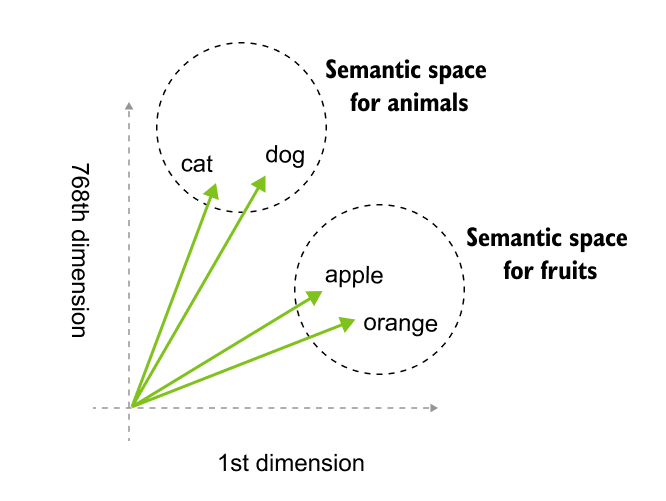
Figure 1.26 high-dimensional embeddings transform semantic meaning into geometric coordinates. In this 768-dimensional space, linguistic relationships are defined by proximity, grouping concepts like animals and fruits into distinct neighborhoods.
The breakthrough came from the distributional hypothesis: words appearing in similar contexts tend to have similar meanings. If “coffee” frequently appears near “morning,” “cup,” and “brew,” while “tea” appears near similar words, a model can learn that coffee and tea are related concepts. Word2Vec revolutionized this approach by training neural networks to predict words from context (CBOW) or context from words (Skip-gram). Through millions of training examples, the network’s hidden layer learns to position similar words near each other in vector space. After training, “king” naturally clusters near “queen” and “prince,” while “banana” groups with “apple” and “fruit.” Most remarkably, these embeddings capture analogical relationships geometrically: the vector arithmetic “king - man + woman” yields a vector nearly identical to “queen,” demonstrating that the model has learned abstract concepts like gender and royalty as directions in space.
Embeddings in Large Language Models
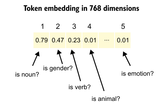
Figure 1.27: Dense embedding vectors transform token IDs into high-dimensional representations where specific dimensions encode learned semantic features. This layer functions as a learned lookup table that maps tokens to unique vectors, enabling the model to capture nuanced semantic attributes like parts of speech or categorical relationships.
Modern LLMs transform token IDs into dense embedding vectors, typically ranging from 768 to 4096 dimensions, where each dimension encodes aspects of meaning learned during training. Unlike Word2Vec’s static embeddings where each word has one fixed representation, transformer models employ contextual embeddings that dynamically adjust based on surrounding tokens. The word “bank” receives different vector representations when appearing in “river bank” versus “investment bank,” enabling the model to disambiguate meaning through context. These embeddings are learned end-to-end during training, with the model discovering optimal representations that maximize its ability to predict the next token. The embedding layer becomes a learned lookup table that maps each of the 50,000+ token IDs to a unique vector in high-dimensional space, where semantic similarity translates to geometric proximity.
The power of LLM embeddings lies in their ability to encode multiple layers of linguistic information simultaneously. Each vector captures semantic meaning (cat near dog), syntactic roles (verbs clustering separately from nouns), conceptual relationships (similar terms grouping together), and even abstract patterns like sentiment or formality. Through billions of training examples, the model learns to position tokens in this space such that vector operations correspond to meaningful transformations. This geometric structure enables transformers to perform complex reasoning by manipulating these vectors through attention mechanisms and feed-forward networks, turning language understanding into mathematical computation.
However, embeddings alone cannot capture the sequential nature of language, where word order fundamentally changes meaning. This limitation leads us to positional embeddings, which encode each token’s location in the sequence, enabling transformers to understand that “dog bites man” differs crucially from “man bites dog.”
Positional Embedding
The Need for Positional Information
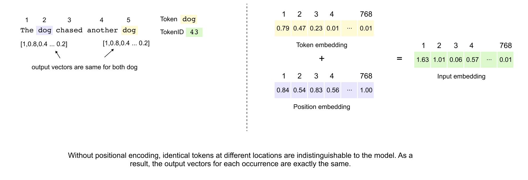
figure 1.28: Positional embeddings introduce sequential context into the Transformer architecture by adding unique position-aware vectors to token embeddings. This summation allows the model to distinguish identical tokens appearing at different sequence locations, enabling the architecture to capture syntactic and referential relationships despite its inherently parallel, set-based processing nature.
In natural language, word order fundamentally shapes meaning. Consider the sentences “The dog chased the cat” versus “The cat chased the dog.” While both sentences contain identical words, their meanings differ entirely based on word positioning. Traditional sequential models like RNNs inherently capture this ordering through their recurrent nature. However, the Transformer architecture processes all tokens simultaneously through self-attention, treating input as an unordered set. Without explicit positional information, a Transformer would produce identical representations for “dog” regardless of its position in the sentence, making it impossible to distinguish between different occurrences or understand sequential relationships.
This limitation becomes particularly problematic when dealing with pronouns and references. In “The dog chased the ball but it could not catch it,” the two instances of “it” refer to different entities based solely on their positions relative to other words. To address this fundamental limitation, Transformers incorporate positional embeddings that encode sequence order information directly into the model’s representations.
Integer Positional Encoding: The Simplest Approach
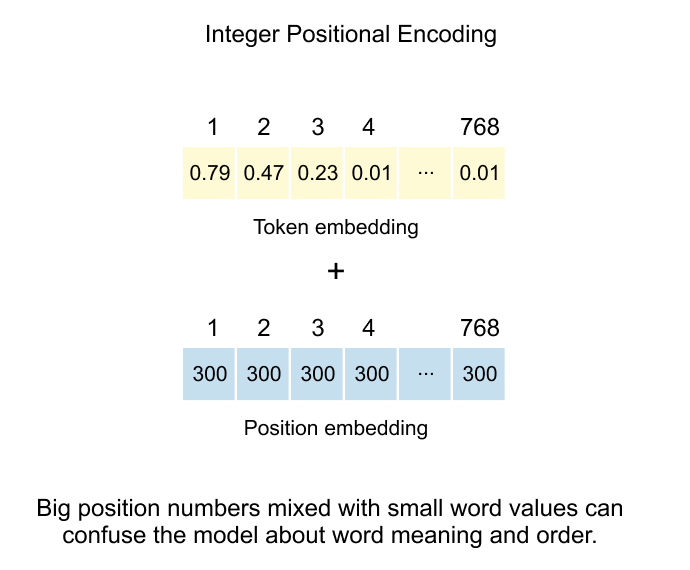
figure 1.29: The additive method of injecting positional data by combining token embeddings with integer-based position vectors, while noting the drawback that large integer values can interfere with and potentially confuse the model regarding the original word's semantic meaning.
The most straightforward solution involves assigning each position a unique integer value. In this scheme, if a token appears at position 300 in the sequence, we create a positional embedding vector where every dimension contains the value 300. This vector, matching the token embedding dimensions, gets added element-wise to the token embedding.
For a concrete example with an 8-dimensional embedding space, the token “dog” at position 300 would receive a positional embedding of [300, 300, 300, 300, 300, 300, 300, 300]. The final input representation becomes the sum of the token embedding and this positional embedding.
However, this approach suffers from a critical flaw: scale mismatch. Token embeddings typically contain small values clustered around zero, carefully learned to capture semantic nuances. Position values, especially for longer sequences, can grow arbitrarily large. When position 500 adds [500, 500, ...] to delicate token embeddings with values like [0.23, -0.15, 0.08, ...], the positional signal completely overwhelms the semantic information. The model loses the ability to distinguish between different words, focusing instead on their positions.
Binary Positional Encoding: Constraining the Range
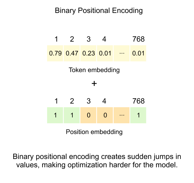
figure 1.30: This technique represents positions using binary bit strings to keep values between 0 and 1, but it creates sudden jumps in the embedding space that complicate the training process for the model.
To address the magnitude problem inherent in integer encoding, binary positional encoding represents positions using their binary representation, naturally constraining all values between 0 and 1. This approach transforms each position number into its binary form and uses those bits directly as the positional embedding vector.
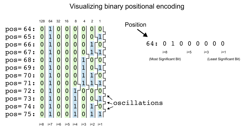
Figure 1.31: This demonstrates how binary representations change across consecutive integer positions. It highlights the rapid bit flipping in the least significant bit position which creates frequency oscillations that make optimization more difficult for the model.
Consider the visualization showing positions 64 through 75 with their 8-bit binary representations. Position 64, which equals 01000000 in binary, becomes the embedding vector [0, 1, 0, 0, 0, 0, 0, 0]. Here, each bit position corresponds to a dimension in the embedding space, with i=8 representing the most significant bit (MSB) and i=1 representing the least significant bit (LSB).
Looking at the pattern across consecutive positions reveals a fascinating structure. Position 64 starts with [0, 1, 0, 0, 0, 0, 0, 0]. Position 65 becomes [0, 1, 0, 0, 0, 0, 0, 1], position 66 transforms to [0, 1, 0, 0, 0, 0, 1, 0], and position 67 yields [0, 1, 0, 0, 0, 0, 1, 1]. The rightmost bit (i=1) flips with every single position increment, creating a rapid alternation between 0 and 1.
The second bit from the right (i=2) follows a different rhythm, maintaining its value for two positions before flipping. It stays 0 for positions 64-65, switches to 1 for positions 66-67, returns to 0 for positions 68-69, and so forth. The third bit (i=3) changes every four positions, remaining stable from 64-67, then flipping for 68-71.
This creates a hierarchical encoding scheme where each bit position operates at a different frequency. The LSB oscillates most rapidly, capturing fine-grained positional differences between adjacent tokens. Moving leftward through the bits, oscillation frequencies decrease exponentially. The fourth bit changes every 8 positions, the fifth every 16 positions, the sixth every 32 positions, and the seventh every 64 positions. The MSB (i=8) remains constant for 128 consecutive positions before flipping.
In the visualization, this pattern becomes immediately apparent. The rightmost column shows constant flickering between (0) and (1) for every position. The i=2 column displays pairs of same cells. The i=3 column shows groups of four, and this doubling pattern continues across all dimensions. The leftmost column (i=8) remains uniformly across the entire visible range, as positions 64-75 all share the same MSB value of 0.
This encoding elegantly solves the scale problem that plagued integer encoding. Instead of values potentially reaching into the thousands, every dimension now contains either 0 or 1. When added to token embeddings clustered around zero, these binary values preserve the semantic information while injecting positional signals at a comparable scale.
The hierarchical structure provides the model with positional information at multiple granularities simultaneously. Lower-indexed dimensions encode local sequential relationships, helping the model understand which tokens appear near each other. Higher-indexed dimensions capture global positional context, indicating whether tokens appear in the first half versus second half of the sequence, or in early versus late quarters.
However, binary encoding introduces a critical limitation: discontinuity. The hard transitions between 0 and 1 create step functions rather than smooth gradients. When the model needs to learn relationships between positions 67 ([0, 1, 0, 0, 0, 0, 1, 1]) and 68 ([0, 1, 0, 0, 0, 1, 0, 0]), multiple dimensions flip simultaneously. These abrupt changes complicate gradient-based optimization, as the loss landscape contains sharp edges and discontinuous regions.
During backpropagation, these discrete jumps prevent smooth gradient flow. Small parameter updates cannot gradually transition the model’s understanding between binary states. The optimizer must navigate around these discontinuities, potentially getting stuck in suboptimal configurations or requiring careful learning rate scheduling to handle the non-smooth optimization landscape.
Despite these challenges, binary encoding demonstrates the key insight that positional information can be encoded through patterns of oscillation at different frequencies. This conceptual breakthrough, showing that different dimensions can operate at different temporal scales, directly inspired the development of sinusoidal positional encoding, which maintains these beneficial oscillatory patterns while ensuring continuous, differentiable representations throughout the embedding space.
Sinusoidal Positional Encoding: Continuous Representations
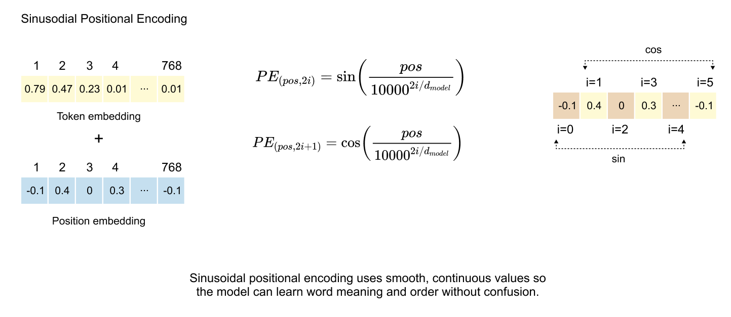
Figure 1.32: Sinusoidal PE applies trigonometric sine and cosine functions to generate continuous and bounded positional vectors, which enables the model to learn sequential relationships while avoiding the optimization challenges and discontinuities inherent in integer and binary positional encodings.
The breakthrough in positional encoding came with the sinusoidal approach, introduced in the seminal “Attention Is All You Need” paper. This method preserves the oscillatory patterns discovered in binary encoding while ensuring smooth, continuous values bounded between -1 and 1, eliminating the discontinuity problems that hindered optimization.
The Mathematical Foundation
The sinusoidal formulation employs alternating sine and cosine functions across dimensions:
Where pos denotes the token’s position in the sequence, i represents the dimension index, and d_model indicates the total embedding dimensionality. The constant 10000 serves as the base for creating a geometric progression of wavelengths across different dimensions.
Frequency Spectrum Analysis
Taking GPT-2’s architecture as an example, with d_model = 768 and maximum context length = 1024, we can observe how different dimensions encode positional information at varying frequencies. For any given position, we compute 768 values using the alternating sine-cosine formulas.
At the lowest dimension (i=0), the formula simplifies to sin(pos/1) = sin(pos), creating rapid oscillations. The adjacent dimension uses cos(pos/1) = cos(pos). As the dimension index increases, the denominator 10000^(2i/768) grows exponentially, progressively slowing the oscillation frequency.
Sinusoidal Patterns Across Different Dimensions
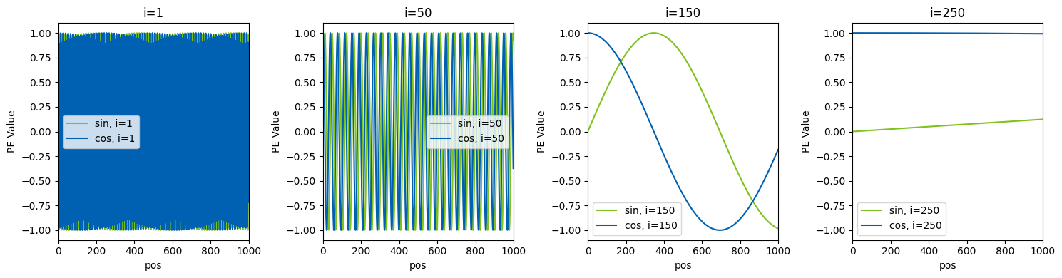
Figure 1.33: The visualization reveals how positional encodings behave across four different dimension indices:
At i=1, both sine and cosine components oscillate extremely rapidly, appearing as dense vertical lines that alternate between approximately -1 and 1. This high-frequency pattern changes with nearly every position, capturing fine-grained local relationships between adjacent tokens.
At i=50, the oscillation frequency decreases noticeably. The sine and cosine waves create regular patterns with periods spanning roughly 20-30 positions. These medium-frequency components encode relationships at the phrase or sentence level.
At i=150, the waves become smooth and gradual, with clear sinusoidal curves visible. The sine (green) and cosine (blue) components maintain their 90-degree phase offset, completing only 2-3 full cycles across the entire 1024-position range. These dimensions capture broader structural information about whether tokens appear in early, middle, or late portions of the sequence.
At i=250, the oscillation becomes extremely slow, with the functions barely completing a single cycle across the full context. The cosine component remains nearly constant around 1, while the sine component stays close to 0, providing stable anchoring for global position context.
Sinusoidal encoding creates a hierarchical representation where each position receives a unique 768-dimensional fingerprint. Lower dimensions oscillate rapidly between positions, capturing local token relationships and word order, while higher dimensions change gradually, encoding broader context like paragraph boundaries and document structure. This combination of multiple sine-cosine pairs at different frequencies generates a unique signature for every position. Unlike binary encoding’s abrupt 0-to-1 transitions, sinusoidal encoding provides smooth, continuous functions that enable stable gradient flow during backpropagation, dramatically improving training efficiency. The bounded range between -1 and 1 keeps positional signals at a scale comparable to token embeddings, preventing positional information from overwhelming semantic content while allowing the optimizer to make incremental refinements.
The sinusoidal approach offers significant practical advantages: it requires no learned parameters, reducing model complexity and training overhead, and its mathematical formulation naturally extends to arbitrary sequence lengths, potentially enabling generalization beyond training context sizes. In practice, positional encodings are precomputed for the maximum sequence length and stored as a lookup table. During processing, these encodings are retrieved and added element-wise to token embeddings, preserving semantic information while injecting positional signals. This simple yet elegant solution simultaneously addresses multiple challenges: maintaining bounded values, ensuring smooth optimization, providing unique position identification, and encoding multiscale temporal information. These properties have established sinusoidal positional encoding as a cornerstone of the Transformer architecture, inspiring numerous variations while remaining widely used in its original form across modern language models.
1.6 Transformer Block
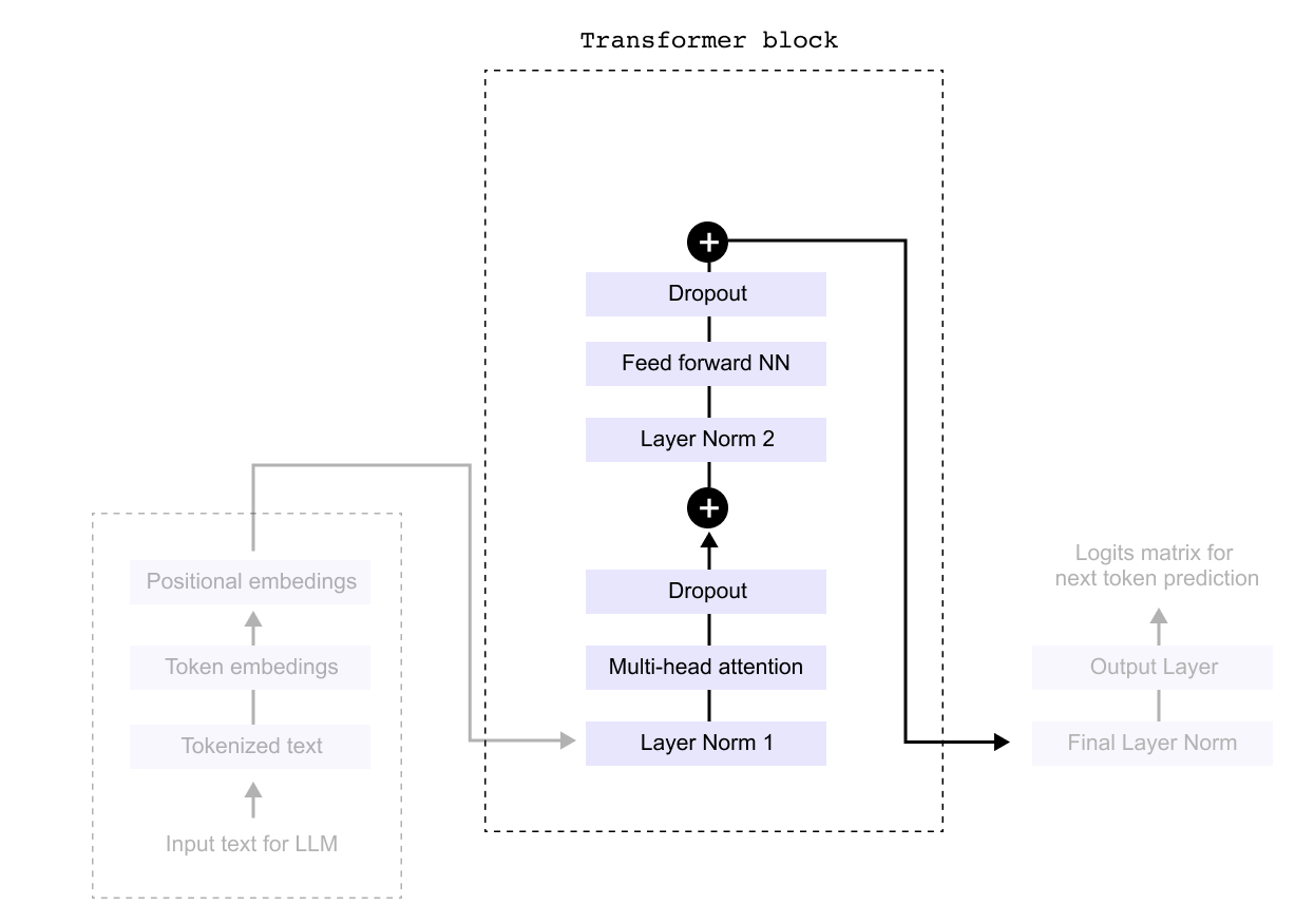
Figure 1.34 Inside the transformer block: multi-head attention, feed-forward network, layer normalization, and dropout layers work in sequence to process token representations
Having converted our raw text into meaningful numerical representations through tokenization and embeddings, we now enter the heart of the language model: the Transformer Block. This is where the real magic happens. The block contains several components working in sequence, including layer normalization, dropout layers, and feed forward networks. However, before we dive into these supporting elements, we need to understand the star of the show: the attention mechanism. The multi head attention layer is what gives transformers their remarkable ability to understand context and relationships between words, no matter how far apart they appear in a sentence. Once we grasp how attention works and explore the feed forward network that follows, we can then circle back to understand how the other components like dropout and layer normalization help stabilize and improve the overall system. For now, let’s focus on what makes transformers truly powerful: their attention mechanism.
1.7 The Need for Attention Mechanism
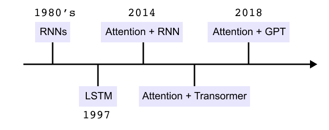
Figure 1.35 Timeline of sequence modeling methods from early RNNs to LSTMs, attention with RNNs, transformers, and GPT models.
Feedforward neural networks see every input as independent. For a sentence such as “The cat sat on the mat” the model processes each word separately and has no built in notion of order or context. This is not enough for language, where meaning depends on how words are arranged.
Recurrent neural networks introduce a hidden state that is passed along the sequence. The encoder reads tokens one by one, updates its hidden state at each step, and hands the final state to a decoder. The decoder must use this single vector as a summary of the entire input sentence. As sequences get longer, early information is squeezed into this fixed size state and gradually fades. This is the context bottleneck.
LSTMs improve the situation with a cell state and gates that control what to store and what to forget. They maintain information over longer spans than basic RNNs, but they still process tokens step by step and still rely on compressed hidden states. Long sentences can still overwhelm this bottleneck.
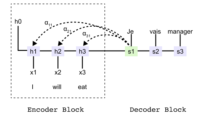
Figure 1.36: Encoder-decoder RNN for the sentence “I will eat” showing encoder hidden states h1, h2, h3 and decoder states that must rely on a single summary vector.
To see the bottleneck more concretely, consider an encoder decoder model that translates the English sentence “I will eat into French”. The encoder produces hidden states h1, h2, h3 for the three input tokens and a final state that is passed to the decoder. Without attention, the decoder can only use this final state when generating the first French word. It has no direct way to reach back to h1 or h2.
Attention
Attention removes the hard bottleneck by giving the decoder direct access to all encoder states. At each decoding step the model compares the current decoder state with every encoder state and produces attention scores. After a softmax these scores become attention weights that sum to one.
The decoder then forms a context vector as a weighted sum of the encoder states. If the first input word is most relevant for the current output, its weight may be close to one while the others are close to zero. At the next step the weights are recomputed and the model can shift its focus to a different part of the sentence.
In the translation example, when the decoder produces the first French word it might focus almost entirely on h1. When it moves on to the second French word it can focus more on h2, and so on. Instead of depending on a single final state, the decoder now has a flexible view over the entire input sequence at every step.
Bahdanau attention
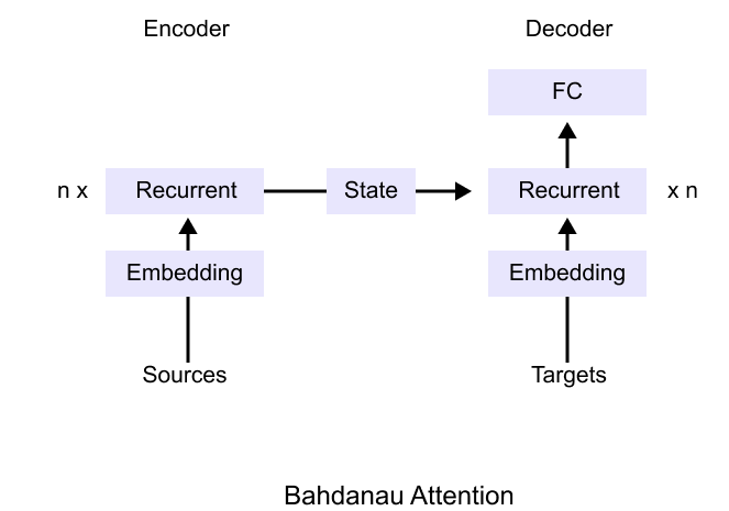
Figure 1.37: Bahdanau attention architecture: the encoder produces a sequence of states and the decoder combines its own state with a context vector formed as a weighted sum of all encoder states
Bahdanau attention was the first widely adopted implementation of this idea. The encoder is still a recurrent network that produces a sequence of hidden states. The decoder is also recurrent, but before predicting each target token it computes alignment scores between its current state and every encoder state. These scores become attention weights, and their weighted sum is the context vector used for prediction.
The attention weights can be visualized as a matrix whose rows correspond to target words and columns correspond to source words. Each cell shows how strongly the model attends to a particular source word when generating a particular target word. This view reveals attention as a soft alignment between the two sentences.
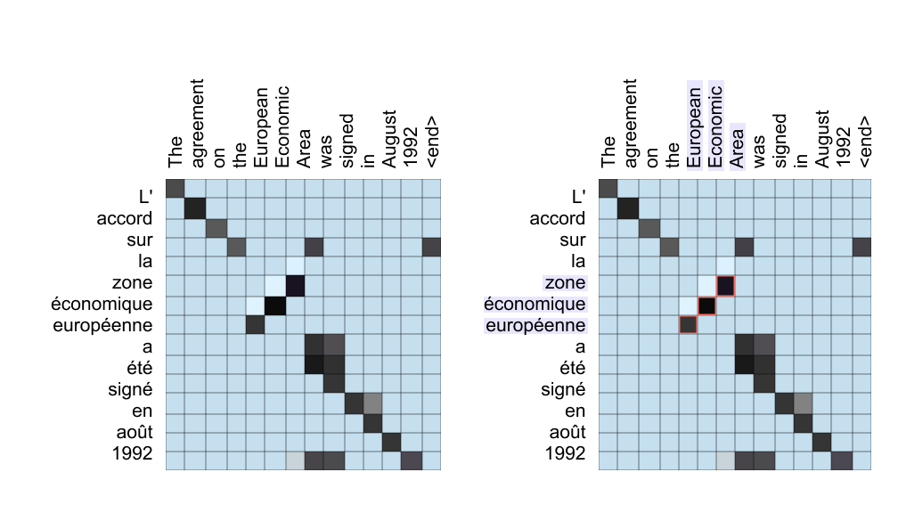
Figure 1.38: Attention heatmaps for a French-to-English sentence pair. The left grid shows overall alignments; the right grid highlights how the model focuses on “European Economic Area” when generating “zone economique europeenne,” capturing word reordering.
These heatmaps show that many words align along a near diagonal, indicating similar order in both languages. Off diagonal patterns reveal reordered phrases. For example, the French adjective corresponding to European appears last in the phrase, but its attention weights point back to the first English word. This ability to align by meaning rather than position is what allows attention based models to handle flexible word order and long range dependencies.
Finally, it is helpful to remember where this attention block lives inside the full transformer model from earlier chapters. The transformer encoder and decoder both contain stacked attention and feedforward sublayers that operate on token and positional embeddings.
We are now ready to see why attention became the central idea in modern language models. Starting from simple recurrent networks and LSTMs, we saw how the context bottleneck makes it hard to remember all the details of a long sentence. Bahdanau attention solved this by letting the decoder look back at every encoder state and learn soft alignments between source and target words, which we visualized through attention weights and heatmaps. So far, attention has connected two different sequences, such as English and French sentences. In the next section we will study self attention in detail and see how letting every token attend to every other token becomes the core operation of the transformer.
1.8 Self Attention Mechanism
What does Self Attention actually means ?
Now that we understand the mechanics of attention, let’s clarify what makes self-attention special, the key concept behind modern language models like Transformers.
Two Types of Attention
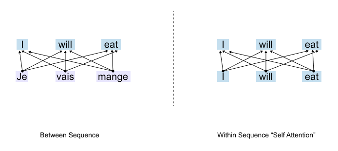
Figure 1.39: Two types of attention: cross-attention connects words across different sequences (e.g., translation), while self-attention connects words within the same sequence.
To understand self-attention, we first need to see where attention was used before. There are two fundamental ways attention can work:
Between Sequences: Attention connects words across different sequences, think of translating from one language to another.
Within a Sequence: Attention connects words within the same sequence to capture relationships and context.
Attention in Translation
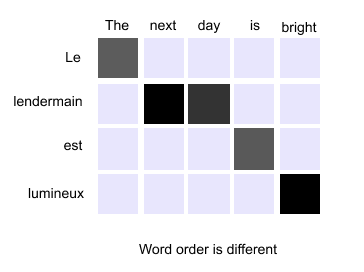
Figure 1.40: Cross-attention in translation: the English phrase “The next day is bright” is aligned to its French counterpart, with attention determining which source words correspond to which target words.
In traditional translation tasks, attention operates between two sequences. Imagine translating the English phrase “The next day is bright” into French. The word order might change. “Day” might align with “jour,” but its position in the French sentence could be different. Attention helps the model figure out these cross-language alignments, which English word corresponds to which French word. This works beautifully for translation. But what happens when we’re not translating at all?
Enter Self-Attention
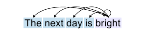
Figure 1.41: Self-attention: every word in a single sentence attends to all other words in that same sentence to build contextual understanding.
Consider a different task: predicting the next word in a sentence. Or understanding what a pronoun refers to. Or simply trying to grasp the meaning of a sentence. Here, we don’t have two separate sequences. We have just one, the sentence itself. This is where self-attention comes in.
Self-attention means that every word in a sentence attends to all other words in that same sentence. Instead of looking across two different sequences (like English and French), the model examines how words relate to each other within a single sequence. The word “day” attends to “next,” to “bright,” to “the”, to everything in its own sentence. It’s attention turned inward. The sequence attending to itself. That’s why we call it self-attention. We cannot encode these complex relationships directly in the attention mechanism using just the raw input embeddings. The connections between words depend on context, grammar, meaning, and a dozen other subtle factors that shift from sentence to sentence.
So what do we do when faced with complexity we can’t hard-code? We let the model learn it. We leave it to weight matrices that can be trained. Before we dive into the mechanics, let’s be clear about our goal. We start with input embeddings, numerical representations of words. But here’s what we want to end up with: context vectors.
What’s the difference?
An input embedding represents a word in isolation. The embedding for “bank” is always the same, whether you’re talking about a financial institution or the side of a river. But a context vector represents a word as it appears in a specific sentence, infused with information from the words around it.
Think about
“The dog chased the ball but it could not catch it.”
The input embedding for the second “it” doesn’t know what “it” refers to, it’s just a generic representation. But the context vector we’re building will carry information from “ball,” from “catch,” from the entire sentence.
Figure 1.42: From input embedding to context vector: the static representation of a word is enriched with information from all surrounding words through self-attention.
It will understand that this particular “it” refers to the ball. So our entire journey with self-attention, the queries, the keys, the attention scores we’re about to explore, all of it serves one purpose: transforming static input embeddings into dynamic context vectors that understand meaning in context.
1.9 Understanding the Input Embedding Matrix
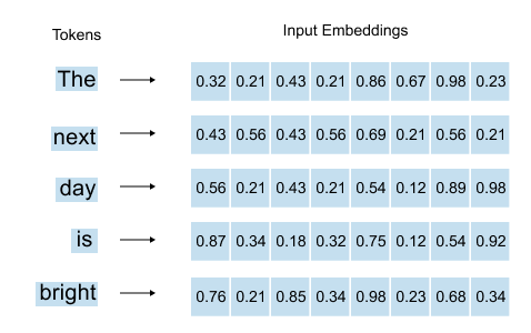
Figure 1.43: For each word, the word embedding and positional embedding are summed to produce the input embedding vector.
As we’ve already seen, for each word in our sentence, we have an embedding vector combined with positional information, that is, the word embedding plus the positional embedding that tells us where the word sits in the sequence. The sum of these two gives us our input embedding vector for each word.
When we stack all these input embedding vectors together for an entire sentence, we get what’s called the input embedding matrix.
Let’s say we’re working with the sentence
“The next day is bright”
that’s five words. Our input embedding matrix would have dimensions (5, 8).
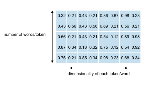
Figure 1.44: The input embedding matrix for the sentence “The next day is bright” has shape (5, 8): five rows (one per word) and eight columns (the embedding dimension).
What do these numbers mean?
The 5 rows come from having 5 words. Simple enough. Each word gets its own row in the matrix. If we had ten words, we’d have ten rows. The number of rows always matches the number of words in our sequence.
The 8 columns represent the dimensionality we’ve chosen for our embeddings. Each word is represented as an 8-dimensional vector, eight numbers that capture its meaning. This dimension is something we decide when building our model. It’s a design choice.
In GPT-2, for instance, the embedding dimension varies: 768 for GPT-2 Small, all the way up to 1,600 for GPT-2 XL. Larger dimensions can capture more nuanced information, but they also require more computation.
The Problem We’re Solving
So here we are with our input embedding matrix. Each word has its 8-dimensional vector. But here’s what’s missing: these vectors exist in isolation. They don’t know about each other.
Look at the word “day” in our sentence “The next day is bright.” Its input embedding vector is just a generic representation of the word “day.” It doesn’t know it should pay attention to “bright.” It doesn’t know that “next” right before it gives it temporal context. It has no idea how much importance it should give to “the” or “is” or any other word in the sentence.
This is exactly why we need to transform input embeddings into context vectors. We need to integrate information from all the other words. We need each word’s representation to reflect not just what it is, but what it means in this particular sentence, surrounded by these particular neighbors. That’s the journey we’re about to take.
Before we can perform any attention calculations, we must first define our input sequence and its corresponding embedding matrix. We will use the PyTorch library to create a tensor that holds this information for our example sentence: “The next day is bright”. Each word is represented by an 8-dimensional vector
Listing 1.1 Defining the input embedding matrix
import torch

words = [’The’, ‘next’, ‘day’, ‘is’, ‘bright’]

inputs = torch.tensor([
    [0.32, 0.21, 0.43, 0.21, 0.86, 0.67, 0.98, 0.23], # The
    [0.43, 0.56, 0.43, 0.56, 0.69, 0.21, 0.56, 0.21], # next
    [0.56, 0.21, 0.43, 0.21, 0.54, 0.12, 0.89, 0.98], # day
    [0.87, 0.34, 0.18, 0.32, 0.75, 0.12, 0.54, 0.92], # is
    [0.76, 0.21, 0.85, 0.34, 0.98, 0.23, 0.68, 0.34]  # bright
], dtype=torch.float32)


print(”Input Embedding Matrix:”)
print(inputs)
print(”\nMatrix Shape:”)
print(inputs.shape)
Running the previous code prints the following output
Input Embedding Matrix:
tensor([
[0.3200, 0.2100, 0.4300, 0.2100, 0.8600, 0.6700, 0.9800, 0.2300],  [0.4300, 0.5600, 0.4300, 0.5600, 0.6900, 0.2100, 0.5600, 0.2100],
[0.5600, 0.2100, 0.4300, 0.2100, 0.5400, 0.1200, 0.8900, 0.9800],
[0.8700, 0.3400, 0.1800, 0.3200, 0.7500, 0.1200, 0.5400, 0.9200],
[0.7600, 0.2100, 0.8500, 0.3400, 0.9800, 0.2300, 0.6800, 0.3400]
])

Matrix Shape:
torch.Size([5, 8])
The output shows our input object is a tensor with a shape of torch.Size([5,8]). This confirms we have a matrix with 5 rows, one for each of our tokens, and 8 columns, representing the 8-dimensional embedding vector for each token. This matrix is the starting point for the self-attention mechanism, but as noted, these vectors exist in isolation and lack any contextual information from their neighbors.
1.10 From Embeddings to Queries, Keys & Values
Here’s where we meet the heart of self-attention: three trainable weight matrices called Queries, Keys, and Values.
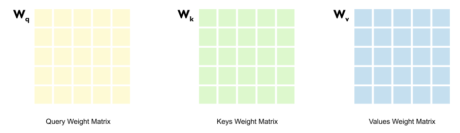
Figure 1.45: The input embedding matrix is multiplied by three separate weight matrices Wq, Wk, and Wv to produce Query, Key, and Value matrices
You might wonder, why three? Why not just use the input embeddings directly?
The answer lies in a fundamental principle of neural networks: they’re universal function approximators. They can learn complex patterns if we give them the right structure. So instead of trying to hand-code how words should relate to each other, we do something smarter.
We initialize three weight matrices with random values at the start. Then we let the training process figure it out. During training, these matrices learn how to transform embeddings in ways that capture meaningful relationships. The Query matrix learns to create vectors that “ask questions.” The Key matrix learns to create vectors that “answer” whether they’re relevant. And the Value matrix? It learns what information should actually be passed along once we know which words matter. We’re not telling the model how attention should work, we’re giving it the tools to learn it on its own.
Let’s understand this by taking one example
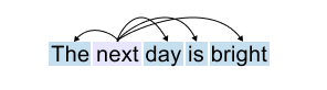
Figure 1.46: The sentence “The next day is bright” with the word “next” highlighted as the current focus of the attention mechanism.
When we focus on a specific word say, “next”.
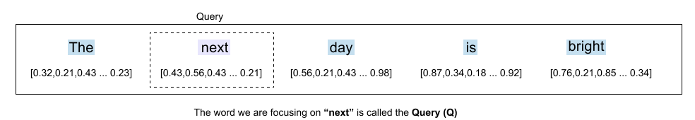
Figure 147: The word “next” acts as the Query, asking how much attention it should pay to each other word in the sentence.
we need to decide how much attention it should pay to all the other words in the sentence. This is where our terminology becomes important. The word we are focusing on (“next”) is called the Query (Q).
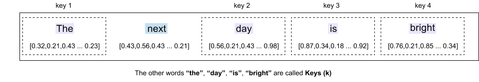
Figure 148: The other words, “the,” “day,” “is,” “bright”, serve as Keys that the query evaluates for relevance.
The other words in the sentence, “the,” “day,” “is,” “bright,” are called Keys (K). These are the words that the query will evaluate. They’re potential sources of information.
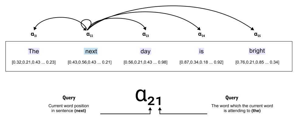
Figure 149: Attention scores α between the query word “next” and all keys. Each score quantifies how strongly “next” should attend to each other word.
Now comes the crucial part: the attention score (α). This score determines how much importance “next” should give to each of these other words. Should “next” pay more attention to “day” (the word right after it) or to “bright” (further away)? The attention scores tell us exactly this.
So “next” uses these attention scores to focus on other words in the sentence, weighing some as more important, others as less so. This is how a word builds its understanding of context.
For example, the attention score α₂₁ means:
“Next” (X₂) is attending to “The” (X₁).
The first 2 represents “next” (position 2 in the sentence).
The second 1 represents “the” (position 1 in the sentence).
The goal of self-attention is to take these attention scores (α values) and use them to modify the original input embeddings, creating context vectors that contain richer information.
Input Embedding (X₂ - “next”): Just represents the word itself.
Context Vector (C₂ - “next”): Now contains information from all relevant words around it, based on attention scores.
Instead of just knowing “next” as an isolated word, the context vector of “next” now understands:
How much “next” relates to “day” (α₂₃)
How much “next” relates to “the” (α₂₁)
How much “next” relates to “is” (α₂₄)
This transformation from input embeddings to context vectors is what makes self-attention so powerful, it helps the model understand relationships between words, not just individual tokens.
Context Vector is an enriched embedding vector. It combines information from all other input elements
The Dimensions of Query, Key, and Value Matrices
Now let’s talk about the actual shape and size of these weight matrices. Understanding their dimensions is crucial to grasping how self-attention works mathematically.
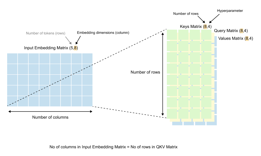
Figure 1.50: Dimensions of the weight matrices: Wq, Wk, and Wv each have shape (d_in, d_out), where din matches the embedding dimension and d_out is a design choice.
If we look at the dimensions of the Query, Key, and Value matrices (Wq, Wk, and Wv), we’ll notice something interesting.
The number of rows in each of these matrices equals the number of columns in our input embedding matrix. Remember, our input embedding matrix has dimensions (5, 8), where 8 is our embedding dimension. So our weight matrices will have 8 rows.
The number of columns in these weight matrices, however, can be anything we choose. This is a design decision.
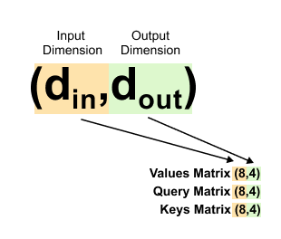
Figure 1.51: The terminology d_in and d_out: din = 8 is the input embedding dimension, and d_out is the chosen output dimension for queries, keys, and values.
When coding language models like GPT-2 or GPT-3, we use specific terminology for these dimensions:
d_in (Input Dimension): The dimension of our input embeddings. In our example, this is 8.
d_out (Output Dimension): The dimension we want for our query, key, and value vectors. This is the number of columns in our weight matrices.
Here’s an important point: you can choose any value for d_out. In practice, it’s often set equal to d_in for simplicity. So if our input dimension is 8, we might set the output dimension to 8 as well. But we don’t have to. In our example, we’re using d_out = 4. Why? To demonstrate that the output dimension is flexible. You have the freedom to choose what works best for your model.
Listing 1.2: Extracting a Token Embedding and Setting Dimensions
x_2 = inputs[1]          # embedding for “next”
d_in = inputs.shape[1]   # input dimension
d_out = 4                # dimension for Q, K, V in this toy example

print(x_2)
print(d_in)
print(d_out)
Here you select the second row of the input matrix, which is the 8 dimensional embedding for the word “next”. The variable d_in confirms that the embedding dimension is 8, matching the theory. The variable d_out is set to 2, which means each query key and value vector will live in a 2 dimensional space in the following examples. In real models d_out is much larger, but using 2 keeps the printed tensors readable.
Output
tensor([0.4300, 0.5600, 0.4300, 0.5600, 0.6900, 0.2100, 0.5600, 0.2100])
8
4
How These Matrices Learn
Figure 1.52: Weight matrices are initialized with random values and updated during training through backpropagation, learning to produce meaningful query, key, and value representations.
At the beginning, all the values in these weight matrices are initialized randomly. They start with no knowledge of language or attention patterns. But here’s where the magic of training comes in.
As we train the model using backpropagation, these random values gradually update themselves. The matrices learn which transformations help the model understand language better.
They learn how to create query vectors that ask the right questions, key vectors that identify relevant information, and value vectors that carry the right content.
1.11 A Quick Note on Matrix Multiplication
Before we dive into multiplying our embedding matrices, let’s make sure we’re all on the same page about how matrix multiplication actually works. If you already know this, feel free to skip ahead. But if matrices feel a bit fuzzy, stick with me for a moment.
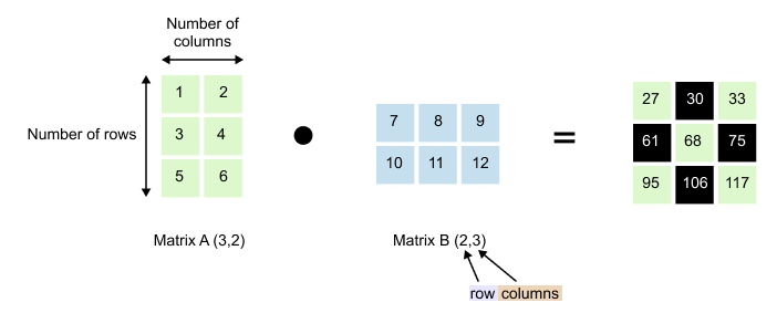
Figure 1.53: Matrix multiplication: Matrix A of shape (3, 2) multiplied by Matrix B of shape (2, 3) produces a result of shape (3, 3). The inner dimensions must match.
We have Matrix A with dimensions (3, 2) and Matrix B with dimensions (2, 3). Notice something important: the number of columns in Matrix A (which is 2) matches the number of rows in Matrix B (also 2). This isn’t a coincidence. For matrix multiplication to work, these inner dimensions must match.
When we multiply them, we get a result with dimensions (3, 3). The outer dimensions survive: 3 rows from Matrix A and 3 columns from Matrix B.
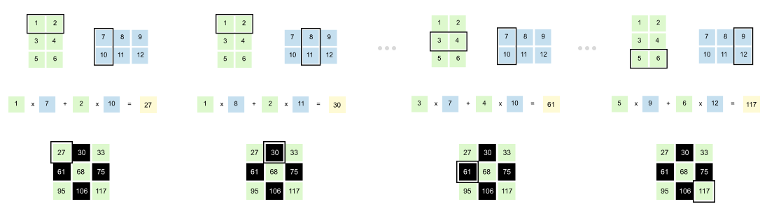
Figure 1.54: Element-wise computation in matrix multiplication: each output entry is the dot product of a row from the first matrix and a column from the second matrix.
To compute each element in the result, you take a row from the first matrix and pair it with a column from the second matrix. Multiply corresponding elements together, then sum them up.
Example: To find the element at position (1, 1):
Take row 1 from Matrix A: [1, 2]
Take column 1 from Matrix B: [7, 10]
Calculate: (1 × 7) + (2 × 10) = 7 + 20 = 27
Another example: For position (2, 1):
Take row 2 from Matrix A: [3, 4]
Take column 1 from Matrix B: [7, 10]
Calculate: (3 × 7) + (4 × 10) = 21 + 40 = 61
You repeat this pattern for every position. Row meets column, multiply and sum. That’s the entire process.
[Step 1] Creating Query, Key, and Value Vectors
The first step in converting our input embedding matrix into context embeddings is straightforward: matrix multiplication. Let’s walk through this process carefully, starting with how we create query vectors.
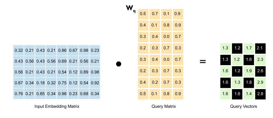
Figure 1.55 The input embedding matrix (5,8) is multiplied by the query weight matrix W_q (8,4) to produce the query matrix (5,4).
We take our input embedding matrix and multiply it by the query weight matrix (W_q). This transformation gives us our query vectors.
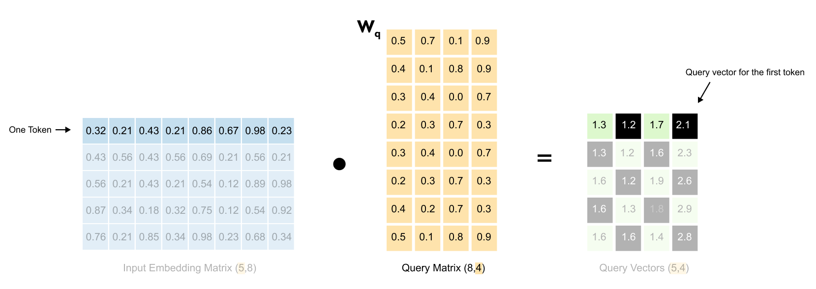
Figure 1.56: Detailed view of the matrix multiplication: each 8-dimensional word embedding is projected through the weight matrix to produce a 4-dimensional query vector
Each row of the input matrix represents one word with its 8-dimensional embedding.
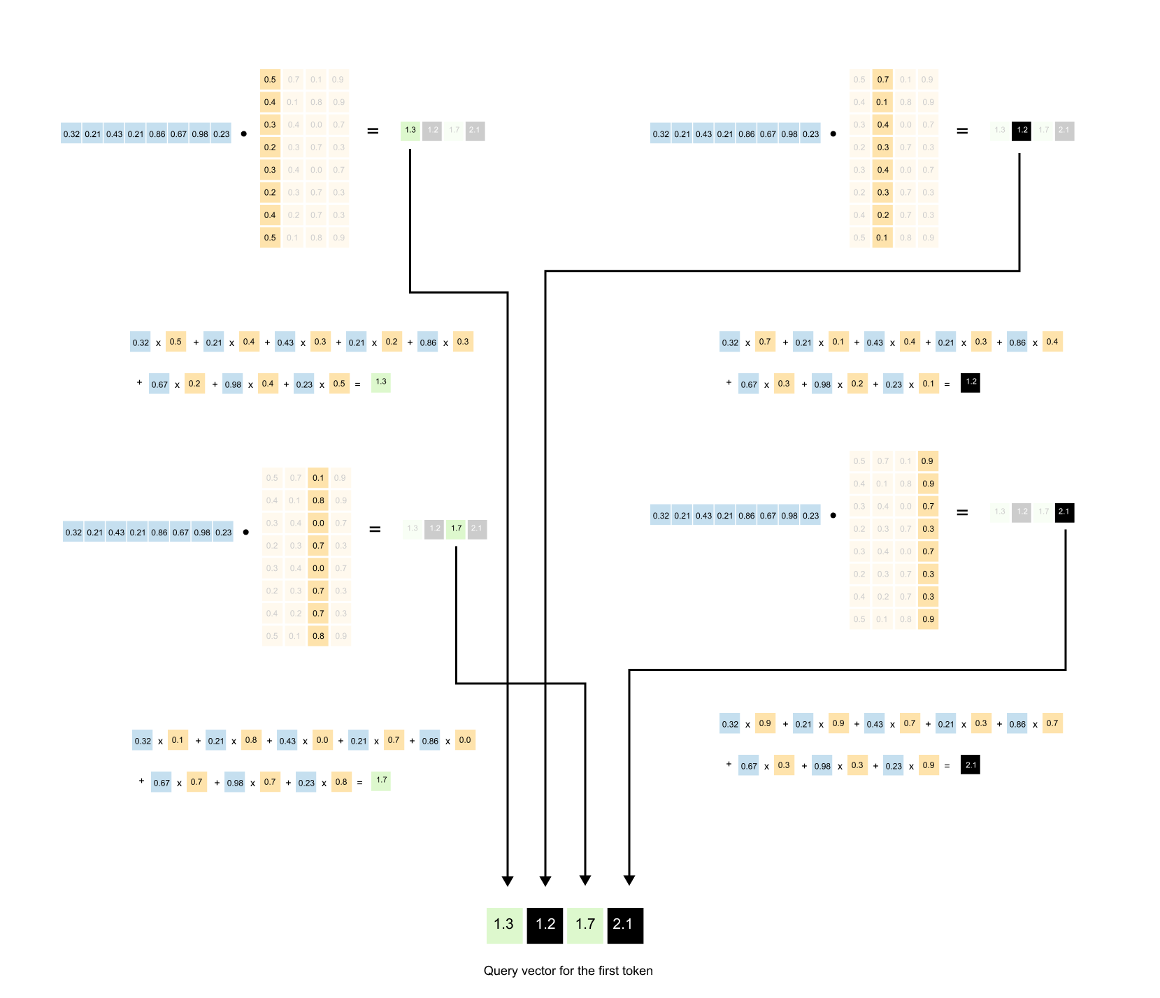
Figure 1.57: Step-by-step computation showing how one row of the input matrix multiplied by W_q produces one row of the query matrix.
When we multiply this row by the weight matrix, we get a new row in the output, a 4-dimensional query vector for that word. This happens for all five words simultaneously.
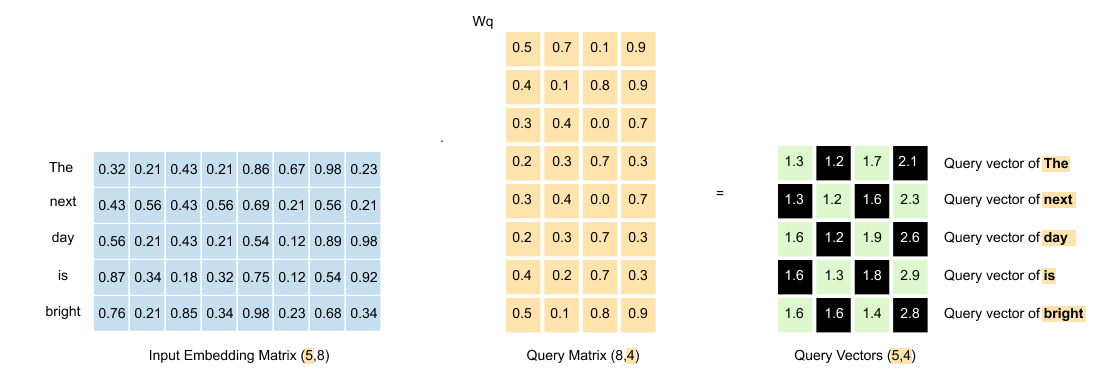
Figure 1.58: The resulting query matrix: five words now have 4-dimensional query vectors, transformed from the original 8-dimensional embeddings.
The result? A query matrix where each of our five words now has its own query vector, transformed from 8 dimensions down to 4.
The Complete Picture
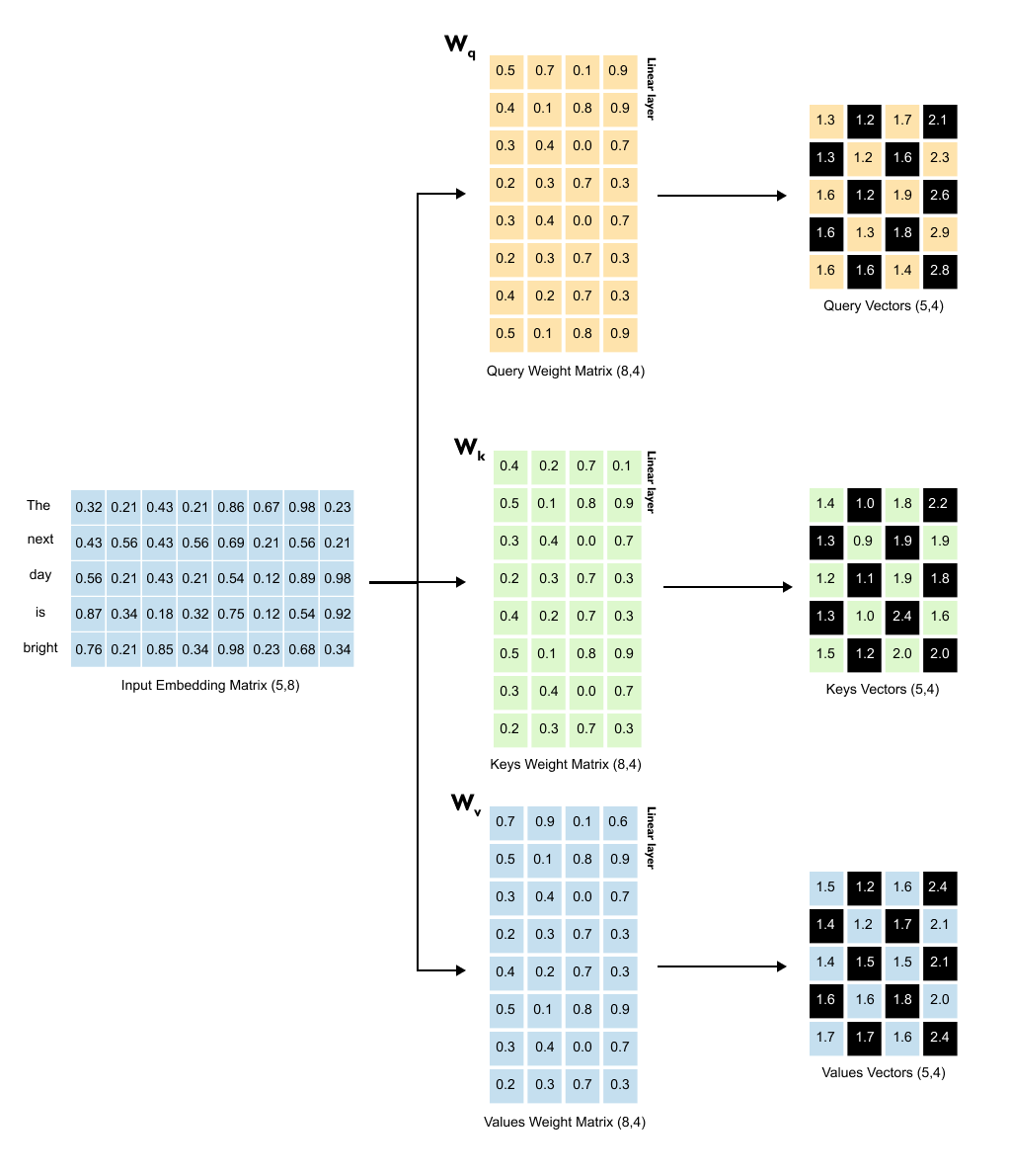
Figure 1.59: All three projections in parallel: the input embedding matrix is multiplied by W_q, W_k, and W_v simultaneously to produce Query, Key, and Value matrices, each of shape (5, 4)
Creating the query vectors is just the beginning. The same transformation process happens two more times, each with its own weight matrix, all operating in parallel.
For the key vectors, we multiply our input embedding matrix by the key weight matrix (W_K). Same dimensions, same process. Each word gets its own key vector.
For the value vectors, we multiply the input embedding matrix by the value weight matrix (W_V). Each word now has a value vector too.
Here’s something important to recognize: we’ve moved from an 8-dimensional space to a 4-dimensional space. More significantly, we’ve moved into a different kind of space altogether. We’re no longer dealing with input embeddings, those static representations of words. We’re now working with query, key, and value vectors. Each lives in its own transformed space, optimized for a specific purpose in the attention mechanism.
This might seem like an odd detour. Why transform our embeddings at all? Why not just work with them directly?
This trick, transforming data into different spaces is fundamental to deep learning, and it’s powerful for a simple reason: sometimes the patterns we need aren’t visible in the original data. Think about it this way. In computer vision, early systems used hand-crafted features like edges and corners. Then convolutional neural networks came along and learned to discover their own features automatically, finding patterns humans never thought to look for. That’s what’s happening here. We’re not stuck with the fixed relationships in our input embeddings. Instead, we let the model learn, through training, what transformations actually help it understand language.
Think of it like passing our input through three different lenses simultaneously. Each lens, each weight matrix transforms the same input embeddings in a different way, extracting different aspects of meaning. When all three transformations are complete, we have three new matrices sitting side by side, all sharing the same dimensions of (5, 4). These three matrices are now ready for the next step in the attention mechanism. The queries and keys will interact to figure out who should pay attention to whom. But that’s a story for the next section.
Listing 1.3 Initializing Query, Key, and Value Weight Matrices
torch.manual_seed(123)

W_query = torch.nn.Parameter(torch.randn(d_in, d_out), requires_grad=False)
W_key   = torch.nn.Parameter(torch.randn(d_in, d_out), requires_grad=False)
W_value = torch.nn.Parameter(torch.randn(d_in, d_out), requires_grad=False)

print(”W_query:”)
print(W_query)
print(”\nW_key:”)
print(W_key)
print(”\nW_value:”)
print(W_value)
Output
W_query:
Parameter containing:
tensor([[ 0.2961,  0.5166, -0.0973,  0.2340],
        [ 0.2517,  0.6886,  0.0451, -0.4128],
        [ 0.0740,  0.8665,  0.3210,  0.0185],
        [ 0.1366,  0.1025, -0.2314,  0.5642],
        [ 0.1841,  0.7264, -0.1035,  0.3399],
        [ 0.3153,  0.6871,  0.2478, -0.1520],
        [ 0.0756,  0.1966,  0.5142,  0.0813],
        [ 0.3164,  0.4017, -0.0879,  0.2904]])

W_key:
Parameter containing:
tensor([[ 0.1186,  0.8274,  0.1040, -0.3055],
        [ 0.3821,  0.6605, -0.2103,  0.1428],
        [ 0.8536,  0.5932, -0.1449,  0.3170],
        [ 0.6367,  0.9826,  0.2553, -0.0872],
        [ 0.2745,  0.6584,  0.0342,  0.5051],
        [ 0.2775,  0.8573, -0.2984,  0.1907],
        [ 0.8993,  0.0390,  0.1206,  0.2843],
        [ 0.9268,  0.7388, -0.0721,  0.3419]])

W_value:
Parameter containing:
tensor([[ 0.7179,  0.7058, -0.1630,  0.3310],
        [ 0.9156,  0.4340,  0.0982, -0.2753],
        [ 0.0772,  0.3565,  0.2056,  0.1468],
        [ 0.1479,  0.5331, -0.0925,  0.2391],
        [ 0.4066,  0.2318,  0.0194,  0.1844],
        [ 0.4545,  0.9737, -0.3086, -0.0417],
        [ 0.4606,  0.5159,  0.1274,  0.0219],
        [ 0.4220,  0.5786, -0.0853,  0.3640]])
This code creates the three trainable weight matrices that turn input embeddings into query, key and value vectors.
The variable d_in is the size of each input embedding, here 8. The variable d_out is the size we want for the query, key and value vectors, here 4.
The tensors W_query, W_key and W_value are wrapped in torch.nn.Parameter, which tells PyTorch that these tensors are learnable weights. During training, gradient descent will update these matrices so that they learn useful transformations.
The shapes printed at the end confirm that each weight matrix has shape 8, 4, matching the description in the theory where the number of rows equals d_in and the number of columns equals d_out.
Listing 1.4: Computing Query, Key, and Value Vectors
queries = inputs @ W_query   # shape: (5, 4)
keys    = inputs @ W_key     # shape: (5, 4)
values  = inputs @ W_value   # shape: (5, 4)

print(”queries.shape:”, queries.shape)
print(”keys.shape   :”, keys.shape)
print(”values.shape :”, values.shape)

print(”\nqueries:”)
print(queries)
print(”\nkeys:”)
print(keys)
print(”\nvalues:”)
print(values)
Output
queries.shape: torch.Size([5, 4])
keys.shape   : torch.Size([5, 4])
values.shape : torch.Size([5, 4])

queries:
tensor([[ 0.8840,  2.0469,  0.3419,  0.5755],
        [ 0.8723,  2.0443,  0.3241,  0.3917],
        [ 0.9738,  1.9925,  0.3154,  0.7673],
        [ 1.1051,  2.1175,  0.2772,  0.9102],
        [ 0.9692,  2.5180,  0.2741,  0.8069]])

keys:
tensor([[ 2.2381,  2.7132,  0.0507,  0.8830],
        [ 2.1564,  2.7927, -0.0064,  0.8684],
        [ 2.6705,  2.7739,  0.0891,  1.0862],
        [ 2.4087,  3.1074,  0.0683,  1.0651],
        [ 2.6735,  3.1745,  0.0538,  1.2434]])

values:
tensor([[ 2.1213,  2.5079, -0.2830,  0.7693],
        [ 2.0476,  2.1981, -0.2301,  0.4927],
        [ 2.1971,  2.4733, -0.2806,  0.9121],
        [ 2.4207,  2.5415, -0.3020,  0.9874],
        [ 2.2625,  2.5902, -0.2714,  0.9625]])
Here we apply the three weight matrices to the full input matrix. Each row of inputs is an embedding for one word.
The matrix multiplication inputs @ W_query takes every word embedding and projects it into query space. The result is a query matrix with shape 5, 4, one query vector of length four for each of the five words. The same happens for keys and values.
This mirrors the explanation in the text that we now have three new matrices, each of size number of tokens, d_out. We are no longer working with raw input embeddings but with transformed representations tailored for searching, being searched and being blended.
[Step 2] Computing Attention Scores
Now that we have our query, key, and value vectors, we’re ready for the heart of the attention mechanism: figuring out which words should pay attention to which other words. Remember, each word has a query vector and a key vector . When we compute the dot product between a query and a key, we get a number that represents how well they align. A high dot product means strong alignment, which translates to high attention. A low dot product means weak alignment, which means less attention.
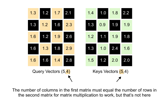
Figure 1.60: The dot product between a query vector and a key vector produces a scalar attention score indicating how well they align.
Here’s where we hit a small technical hurdle. We want to compute all these dot products at once using matrix multiplication. Our Query matrix has dimensions (5, 4) and our Keys matrix also has dimensions (5, 4). If we try to multiply them directly, Query × Keys, we run into a problem. For matrix multiplication to work, the number of columns in the first matrix must equal the number of rows in the second matrix. But Query has 4 columns and Keys has 5 rows. They don’t match. The multiplication simply won’t work. The solution of this problem is to transpose the Keys matrix.
A Quick Note on Matrix Transpose
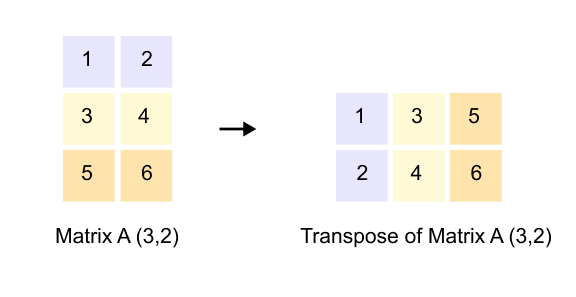
Figure 1.61: Matrix transpose: rows become columns and columns become rows, converting a (3, 2) matrix into a (2, 3) matrix.
If you’re already comfortable with matrix transpose, feel free to skip ahead to the next section. But if transpose feels unfamiliar or you want a quick refresher, stay with me for just a moment.
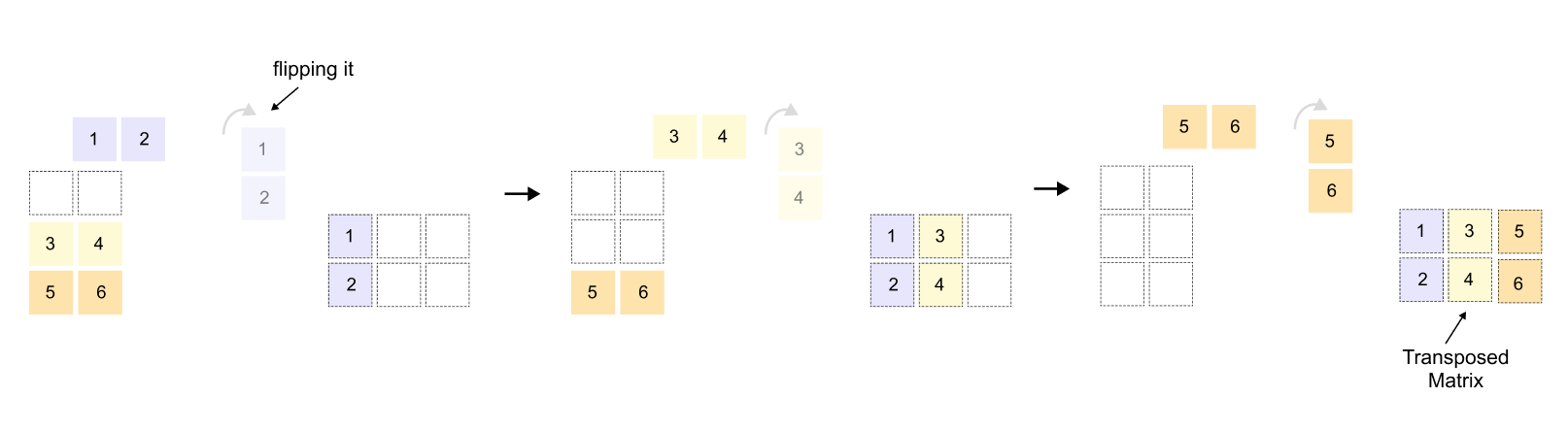
Figure 1.62: Transposing the Keys matrix from (5, 4) to (4, 5) so that it can be multiplied with the (5, 4) Query matrix.
When we transpose a matrix, we flip it along its diagonal. Rows become columns, and columns become rows. If you have a matrix with dimensions (3, 2), its transpose will have dimensions (2, 3). The first row of the original matrix becomes the first column of the transposed matrix. The second row becomes the second column, and so on. It’s like rotating the entire matrix 90 degrees and reflecting it. This simple operation is incredibly useful because it lets us align dimensions for matrix multiplication when they wouldn’t otherwise match.
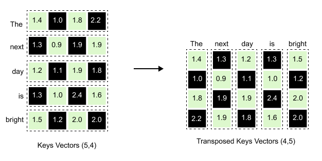
Figure 1.63: The Keys matrix transposed: each word’s key vector becomes a column, converting the (5, 4) matrix into (4, 5).
When we transpose the Keys matrix, each row becomes a column. Notice how the first row for “The” [1.4, 1.0, 1.8, 2.2] in the original Keys matrix becomes the first column [1.4, 1.0, 1.8, 2.2] reading downward in the transposed version. The same happens for every word, ”next” becomes the second column, “day” becomes the third column, and so on, transforming our (5, 4) matrix into a (4, 5) matrix ready for multiplication.
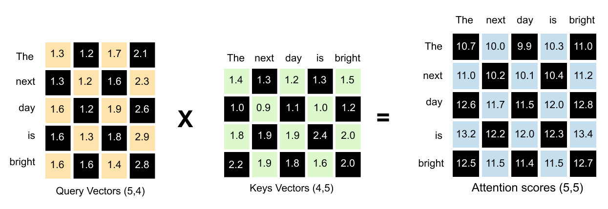
Figure 1.64: Multiplying Query (5, 4) by K_T (4, 5) produces the (5, 5) attention scores matrix, capturing every possible word-to-word relationship.
The result of the dot product of Query and Keys vectors is a (5, 5) attention scores matrix. This matrix captures every possible relationship between words.
Interpreting the Attention Scores Matrix
Now that we have our attention scores matrix, let’s understand what it actually tells us.
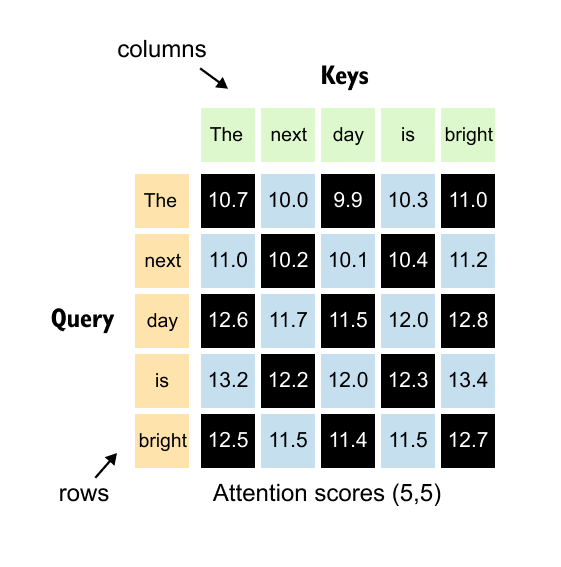
Figure 1.65: The (5, 5) attention scores matrix: rows represent queries and columns represent keys. Entry (i, j) shows how much word i attends to word j.
Each number in this (5, 5) matrix represents how much one word should attend to another word. The key to reading this matrix is simple:
rows represent queries, and columns represent keys.
Let’s look at some concrete examples.

Figure 1.66: Reading the attention matrix: the entry at row 2, column 1 gives the attention score from “next” (query) to “The” (key).
Finding attention between “next” and “The”:
The word “next” is in position 2, so we look at row 2. The word “The” is in position 1, so we look at column 1. The value at position (2, 1) tells us how much “next” attends to “The.”
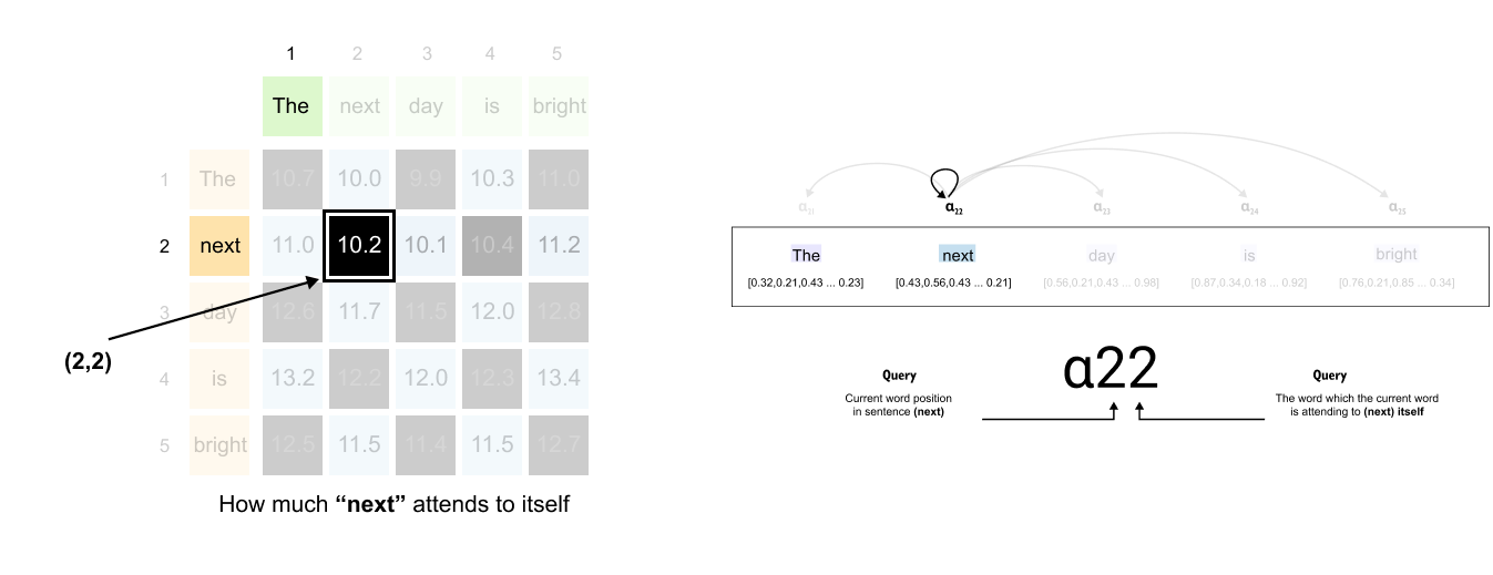
Figure 1.67: The entry at row 2, column 2 shows the self-attention score: how much “next” attends to itself.
Finding attention between “next” and itself:
Same word, but the pattern holds. Row 2 for “next” as the query, column 2 for “next” as the key. The value at position (2, 2) shows how much “next” attends to itself.
Here’s where it gets interesting. Each row tells a complete story about one word’s attention pattern.
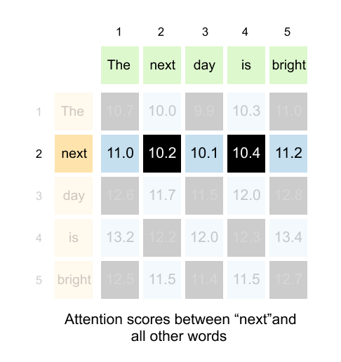
Figure 1.68: Each row tells a complete story about one word’s attention pattern across all other words in the sentence.
Take the second row, for example. This entire row represents the attention scores between “next” (the query) and all other words (the keys). As you move across the columns, you see how much “next” should attend to “The,” then to “next” itself, then to “day,” then to “is,” and finally to “bright.”
The first row does the same for “The.” The third row does it for “day.” Every row follows this pattern.
Problem with Attention Scores Matrix
We have our attention scores matrix, and it captures the relationships between words. But there’s a fundamental issue we need to address. Look at the second row, which represents how much “next” should attend to all other words. The values might be something like 1.3, 0.9, 1.9, 1.9, and 1.2. These numbers tell us relative importance, but they’re hard to interpret.
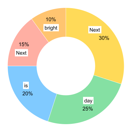
Figure 1.69: Raw attention scores do not sum to one and cannot be interpreted as probabilities. We need normalization to create a proper attention distribution.
What we really want is to make clear, intuitive statements like “next should give 30% of its attention to ‘day,’ 25% to ‘is,’ 20% to itself, 15% to ‘The,’ and 10% to ‘bright.’” We want percentages that sum to 100%, or in mathematical terms, probabilities that sum to 1.
This would let us understand attention as a distribution, like slices of a pie chart, where we can immediately see which words matter most. Right now, our raw scores don’t have this property (11.0 + 10.2 + 10.1 + 10.4 + 11.2), you get 52.9, not 1. The values in each row don’t sum to one, and some might even be negative. We can’t interpret them as percentages or probabilities, and this creates two problems.
First, there’s the interpretability issue. We can’t make clear statements about attention distribution. We can’t say “next pays 22% attention to ‘bright’” when the numbers don’t represent percentages. Second, there’s a training stability issue. When training large language models, it’s better if the numbers stay in a controlled range, ideally between 0 and 1. This makes the training process much more stable. The gradients behave better, and the model learns more reliably.
That’s the problem we need to solve, and the solution is to convert attention scores into attention weights. Attention weights have two key properties: they sum to 1 for each row, and each individual weight lies between 0 and 1. This transformation is called normalization.
A Quick Note on Simple Normalization and Softmax
Simple Normalization
The simplest approach to normalization is straightforward. Take each value in a row and divide it by the sum of all values in that row.
Formula
Example
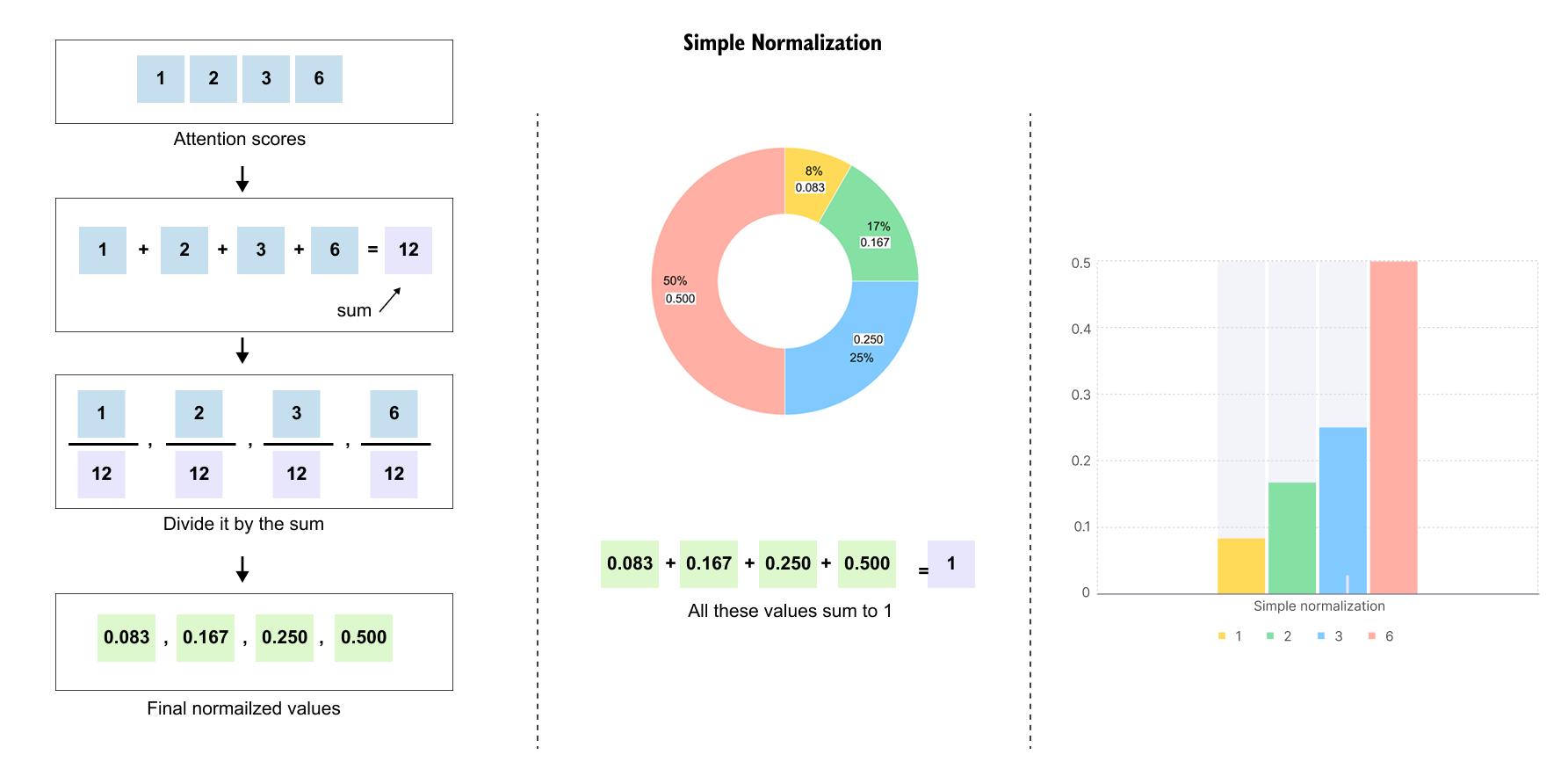
Figure 1.70: Simple normalization divides each value by the row sum, preserving proportions exactly. Softmax exponentiates first, dramatically amplifying differences so the largest value dominates.
These values sum to 1, which is good. The differences are proportional. The value 6 is twice as large as 3, and after normalization, 0.5 is twice as large as 0.25. The proportions are preserved exactly.
Softmax Normalization
Softmax takes a different approach. Instead of dividing by the sum directly, it first exponentiates each value, then normalizes by the sum of exponentials.
Formula
Example
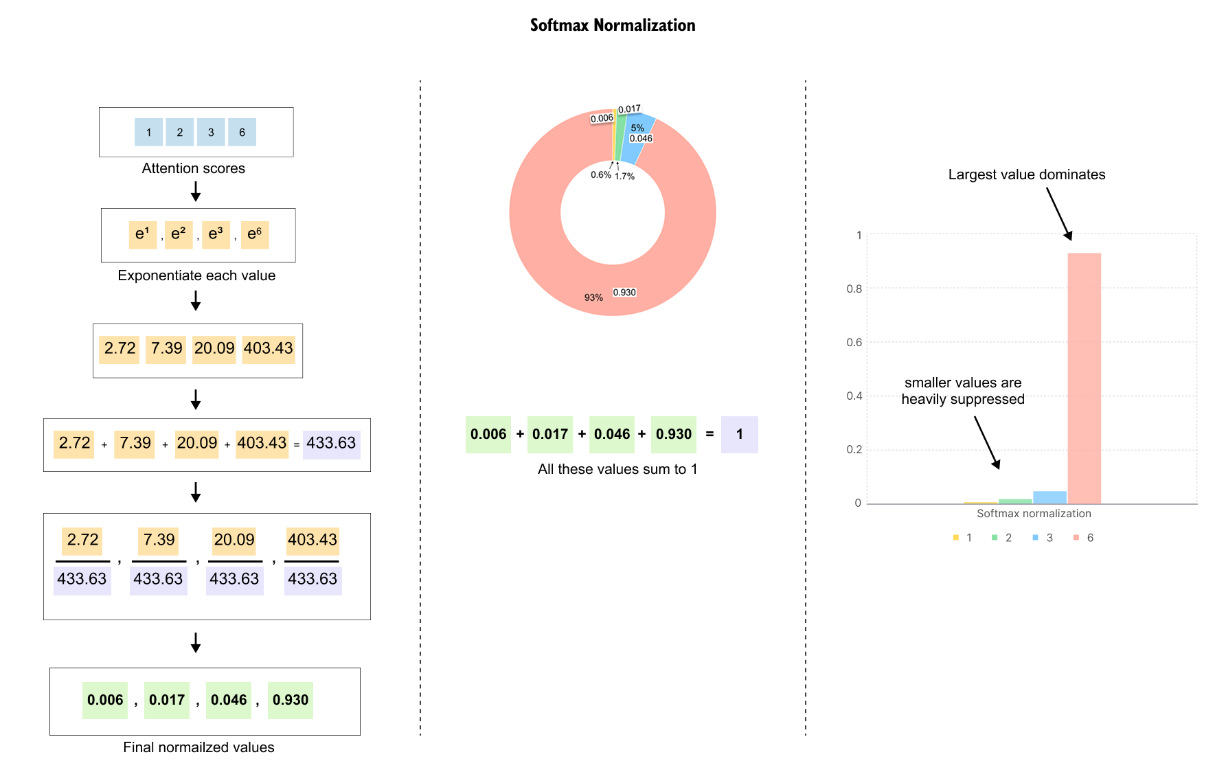
Figure 1.71: Softmax normalization: the largest value (6) receives 93% of the weight while smaller values are heavily suppressed, creating a sharp and decisive attention distribution.
Notice something dramatic. The largest value (6) now dominates completely with 93% of the attention, while the smaller values are heavily suppressed(see the bar graph in the figure). This is the key difference between simple normalization and softmax.
Why Softmax Works Better
Amplification of Differences
Softmax has a crucial property: it amplifies differences. Larger values get disproportionately larger weights, and smaller values get disproportionately smaller weights. This makes the resulting distribution sharper and more decisive.
In our example with simple normalization, the value 6 was six times larger than 1, and after normalization, its weight (50%) was also six times larger than the weight for 1 (8.3%). The proportions stayed exactly the same.
But with softmax, the value 6 gets 93% of the weight, while 1 gets only 0.6%. That’s a ratio of over 150 times! The difference got amplified dramatically. This amplification is exactly what we want in attention mechanisms. When one word should clearly attend to another, softmax makes that relationship strong and clear. The model can make bold, decisive choices about where to focus attention.
Handling Negative Values
Softmax has another important advantage: it handles negative numbers gracefully.
Simple Normalization
We have a problem. A negative probability (-60%) doesn’t make sense. Probabilities must be between 0 and 1.
Softmax
All values are positive! The negative score (-3) simply gets suppressed to nearly zero (0.03%), while the largest value (5) dominates. Softmax automatically ensures all outputs are valid probabilities regardless of input values.
Listing 1.5: Computing Raw Attention Scores
# attention scores for all five tokens
attn_scores = queries @ keys.T     # shape (5, 5)

print(”Attention scores matrix:”)
print(attn_scores)

# attention scores only for the word “next”
idx = 1                            # index 1 is “next”
query_next = queries[idx]          # shape (4,)

keys_T = keys.T                    # shape (4, 5)
attn_scores_next = query_next @ keys_T

print(”\nAttention scores for ‘next’:”)
print(attn_scores_next)
Output
Attention scores matrix:
tensor([[10.3564, 10.4507, 10.9581, 11.3706, 11.7368],
        [10.0395, 10.1182, 10.6117, 11.0026, 11.3353],
        [10.2672, 10.3379, 10.8698, 11.2815, 11.6372],
        [10.5471, 10.6268, 11.1764, 11.5984, 11.9785],
        [11.0007, 11.1326, 11.7058, 12.2208, 12.6405]])

Attention scores for ‘next’:
tensor([10.0395, 10.1182, 10.6117, 11.0026, 11.3353])
The matrix attn_scores contains all raw attention scores before scaling or softmax. Each row corresponds to one query token. Each column corresponds to one key token. Entry (i, j) is the dot product between the query vector for token i and the key vector for token j.
Computing the full matrix in one step is just the matrix form of what we did for a single token earlier. In the second part of the code we select the query for “next” and multiply it with the transposed key matrix. The resulting vector attn_scores_next is simply row one of the full score matrix and shows how strongly “next” matches the key for each word in the sentence, including itself.
[Step 3] Converting Attention Scores to Attention Weight
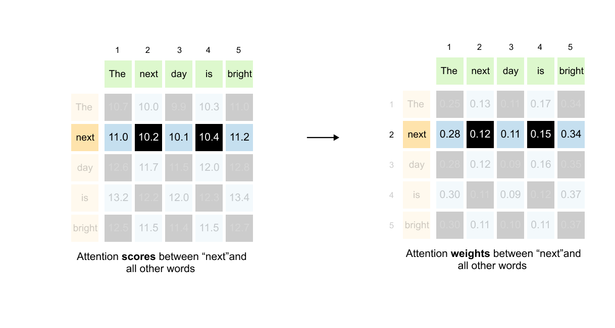
Figure 1.72: Applying softmax row by row converts raw attention scores into normalized attention weights that sum to one, creating an interpretable probability distribution.
Now let’s apply softmax to convert our attention scores into attention weights. We’ll work through this for one row to see exactly how it works.
Looking at our attention scores matrix, let’s take the second row for “next.” The values are:
These represent how much “next” should attend to “The,” “next,” “day,” “is,” and “bright” respectively.
Step 1: Exponentiate each score
Step 2: Calculate the sum
Step 3: Divide each exponential by the sum
Now we can make clear, interpretable statements: “next” pays 33.6% of its attention to “bright,” 27.6% to “The,” 15.2% to “is,” 12.4% to itself, and 11.2% to “day.”
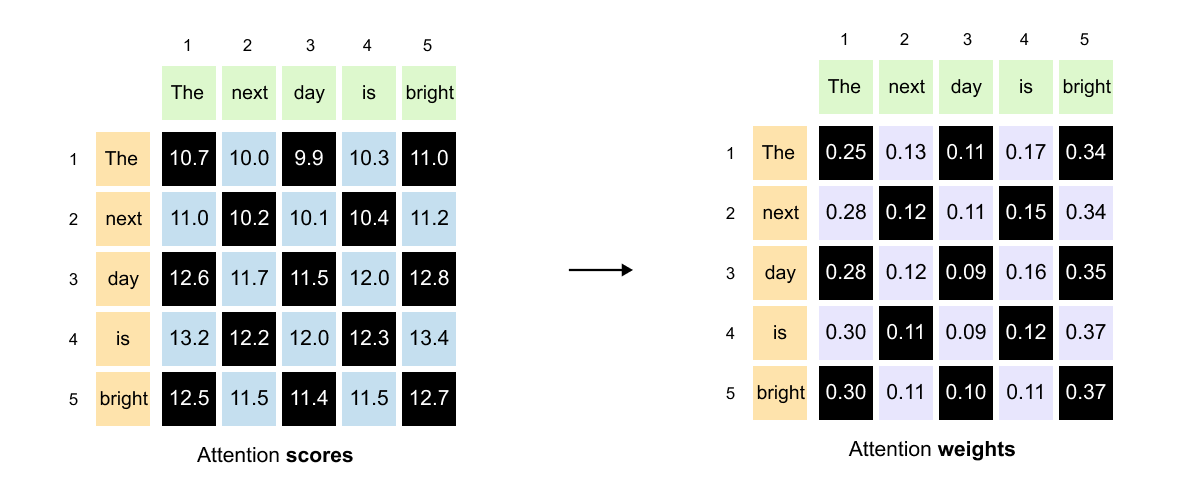
Figure 1.73: The complete attention weights matrix after softmax: every value is between 0 and 1, and every row sums to 1.
We apply this same softmax operation to every row in our attention scores matrix. Each row gets its own independent softmax transformation, converting raw scores into normalized attention weights that sum to 1. The result is our attention weights matrix, where every value is between 0 and 1, every row sums to 1, and we can finally interpret the numbers as meaningful probabilities.
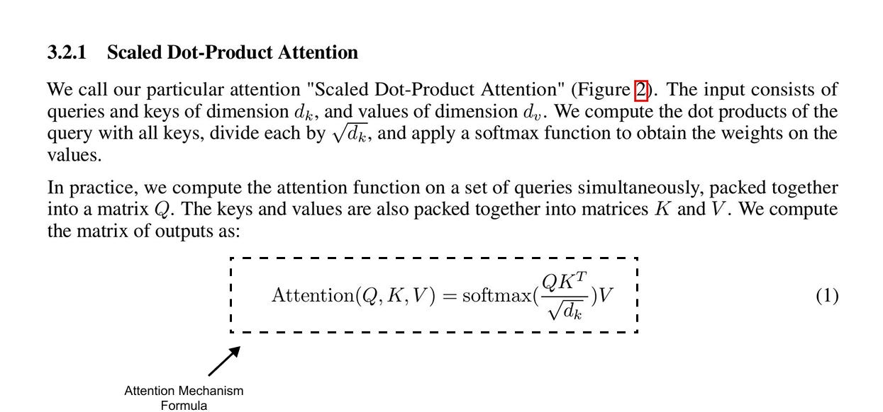
Figure 1.74: The scaled dot-product attention formula from the original transformer paper.
Before we move forward, there’s something important to clarify about the attention formula we’ve been building. What we just covered was the softmax operation, which converts attention scores into attention weights. But in practice, there are two additional operations that happen before we apply softmax: scaling by the square root of the key dimension, and adding a mask.
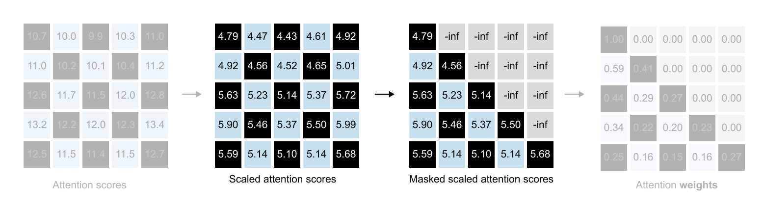
Figure 1.75: The complete attention pipeline: compute QK^T , scale by √ d_k, optionally apply a mask, then apply softmax to obtain attention weights
You might wonder why we’re mentioning this now, after already explaining softmax. The reason is pedagogical. Understanding softmax first makes it much easier to grasp why these additional steps matter. If we had introduced all three operations at once, the picture would have been muddier. By learning them in this order, you’ll see not just what these operations do, but why they’re necessary.
If this sounds a bit abstract right now, don’t worry. The next section will clarify everything. We’ll walk through both scaling and masking step by step, and by the end, you’ll understand exactly how they fit into the complete attention mechanism.
1.12 Why Scale Attention Scores?
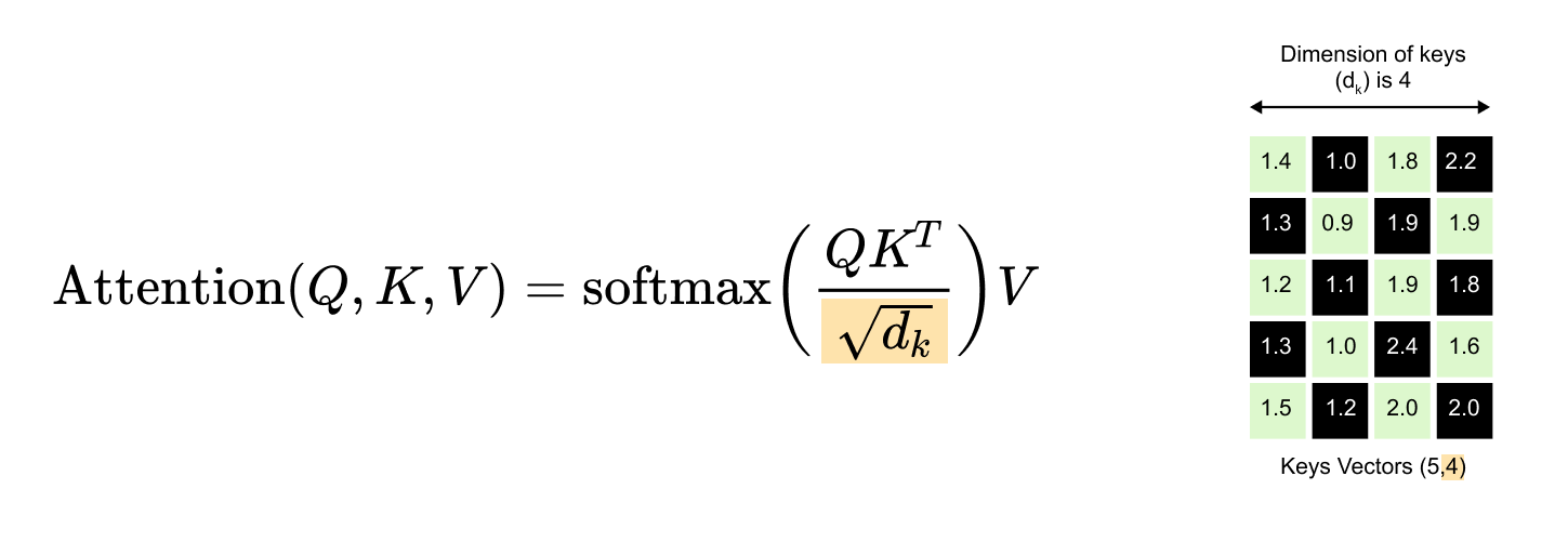
Figure 1.76: The scaling factor normalizes the variance of the dot product, preventing softmax from producing extremely sharp distributions
In the Transformer model, the attention mechanism calculates scores using the formula:
A critical component of this formula is the scaling factor,
This scaling is not arbitrary; it is essential for stabilizing the training process.
The Problem with Unscaled Scores
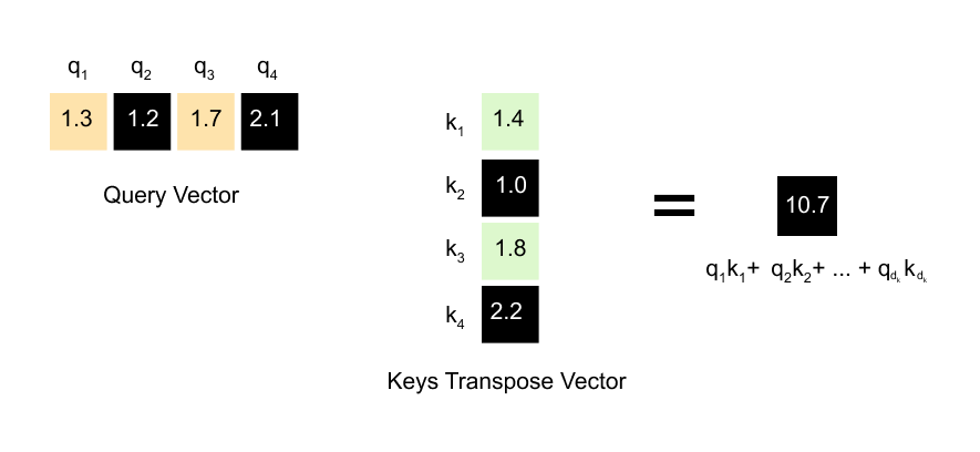
Figure 1.77 : As the key dimension d_k increases, the variance of the dot product grows, causing large scores that push softmax into saturation where gradients vanish.
The attention scores are calculated from the dot product of a query vector (Q) and a key vector (K^T). A dot product is the sum of element wise products:
The problem is that as the dimension (d_k) increases, the variance of this dot product also increases. A larger dimension means more terms are being added together, which can lead to the final scores being very large in magnitude.
These large scores are then passed into the softmax function. The softmax function is sensitive to large inputs. If one score is significantly larger than the others, softmax will assign it a probability very close to 1.0, while all other scores will be assigned a probability very close to 0.0. This is known as saturation.
When this happens, the attention becomes “hard” and “spiky,” focusing on only one position. This makes it difficult for the model to learn, as the gradients during backpropagation become extremely small, effectively vanishing and halting the training process for that attention head.
The Statistical Solution
If we assume the components of (Q) and (K) are independent random variables with a mean of 0 and a variance of 1, then their dot product (Q K^T) will have a mean of 0 but a variance of d_k. To normalize this, we want to scale the dot product so that its variance remains 1, regardless of the dimension d_k.
The standard deviation of the dot product is the square root of its variance, which is
By dividing the dot product (Q K^T) by its standard deviation (, we ensure the input to the softmax function has a stable variance of 1.
Let’s compute the scaled attention matrix
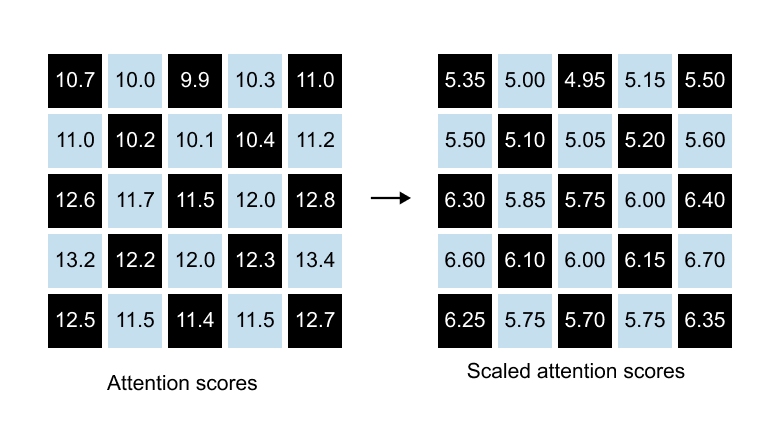
Figure 1.78: Computing the scaled attention scores, key dimension is 4, so √ d_k = 2, and every raw score is divided by 2 before softmax.
“Keys Vectors” a matrix with the shape (5, 4).
This means there are 5 key vectors, and each vector has a dimension of 4.
To get the scaled scores, we must divide every number in “Attention Scores” matrix by our new scaling factor, 2.
This is the “Attention Scores”
Calculation (Dividing by 2):
Final “Scaled Attention Scores” (based on d_k=4):
Listing 1.6: Scaling Scores and Computing Attention Weights
d_k = keys.shape[-1]   # key dimension, 4

# scale scores and convert to attention weights for all tokens

scaled_scores = attn_scores / d_k**0.5
attn_weights = torch.softmax(scaled_scores, dim=-1)

print(”Attention weights matrix:”)
print(attn_weights)
print(”\nRow sums:”, attn_weights.sum(dim=-1))

# same thing, but shown explicitly for the word “next”

scaled_scores_next = attn_scores_next / d_k**0.5
attn_weights_next = torch.softmax(scaled_scores_next, dim=-1)

print(”\nScaled scores for ‘next’:”)
print(scaled_scores_next)
print(”Attention weights for ‘next’:”)
print(attn_weights_next)
print(”Sum of weights for ‘next’:”, attn_weights_next.sum())
Output
Attention weights matrix:

tensor([[0.1331, 0.1401, 0.1781, 0.2413, 0.3074],
        [0.1375, 0.1430, 0.1779, 0.2361, 0.3056],
        [0.1342, 0.1394, 0.1797, 0.2406, 0.3060],
        [0.1307, 0.1352, 0.1776, 0.2426, 0.3139],
        [0.1180, 0.1271, 0.1660, 0.2553, 0.3336]])

Row sums: tensor([1., 1., 1., 1., 1.])

Scaled scores for ‘next’:

tensor([5.0198, 5.0591, 5.3059, 5.5013, 5.6677])
Attention weights for ‘next’:

tensor([0.1375, 0.1430, 0.1779, 0.2361, 0.3056])

Sum of weights for ‘next’: tensor(1.)
Raw dot products can grow large when the key dimension increases and they are difficult to interpret. The first step therefore scales the scores by dividing by the square root of the key dimension d_k. This keeps the variance of the scores roughly constant and prevents softmax from producing extremely sharp distributions.
The call to torch.softmax then turns each row of scaled scores into a proper probability distribution. All entries are between zero and one and each row sums to one, as confirmed by the printed row sums. The attention weight at position (i, j) now expresses the fraction of token i’s attention that is assigned to token j.
For example, the vector attn_weights_next shows how the word “next” distributes its attention across the five tokens. In the example above it puts about thirty percent of its weight on the last word, with the remaining seventy percent spread over the earlier words.
[Step 4] From Attention Weights to Context Vectors

Figure 1.79: The final step of self-attention: multiply the attention weights matrix by the Value matrix to produce context vectors.
Brief Note: The calculations described in this section illustrate the core mechanism of scaled dot-product attention. For simplicity, this example does not apply causal or look-ahead masking, which would be essential in a decoder-based model (like a GPT) to prevent a token from “seeing” future tokens.
In the self-attention mechanism, the final step is to compute the context vector for each token. A common misconception is that attention is applied to the original input embeddings. Instead, attention is used to create a weighted sum of a new, transformed representation of the input. This new representation is called the Value (V) matrix.
The Role of the Value (V) Matrix
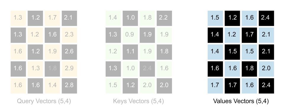
Figure 1.80: The Value matrix is created by multiplying the input embeddings by a separate weight matrix W_V . It provides the representations that are blended according to attention weights.
Just as we created the Query (Q) and Key (K) matrices by multiplying our input embeddings (X) with trainable weight matrices (W_q and W_k), we create the Value (V) matrix by multiplying the input embeddings with its own trainable weight matrix, W_v.
This transformation is crucial. It allows the model to learn a representation of the input tokens that is specifically optimized for constructing the final contextualized output. While the Key matrix is designed for “being searched” and the Query matrix is for “searching,” the Value matrix is designed to “be blended.”
Instead of directly blending the input vectors, we blend these new Value vectors. This gives the model more flexibility and expressive power.
Calculating the Context Matrix
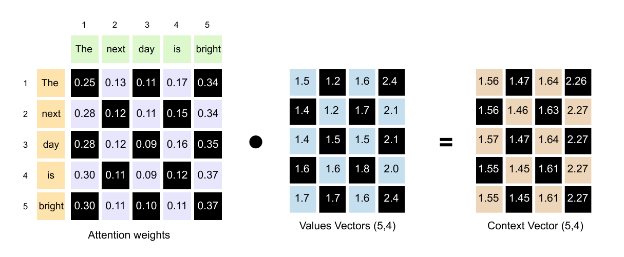
Figure 1.81: The context matrix is computed as a single matrix multiplication: Attention Weights (5, 5) times Values (5, 4) yields the (5, 4) context matrix containing one context vector per token.
The calculation of the final context matrix is a single matrix multiplication:
Let’s break this down using the dimensions from our examples.
1. Attention Weights (A): This is the (5, 5) matrix of normalized scores we calculated previously. Each row (i) of this matrix represents the “attention” that token (i) pays to every other token (including itself).
2. Value (V) Matrix: This is the (5, 4) matrix of transformed input vectors. Each row corresponds to a token, but it now exists in the “value space” with a dimension of 4. The multiplication is therefore:
The resulting (5, 4) Context matrix contains our five new context vectors, one for each input token. Each of these new vectors has a dimension of 4, matching the dimensionality of our value space.
What is a Context Vector?
Each row in the final Context matrix is the new, “context-aware” vector for its corresponding token. This new vector is a weighted sum of all the Value vectors in the sequence. Let’s illustrate by calculating the context vector for the third token, “day” (row 3).
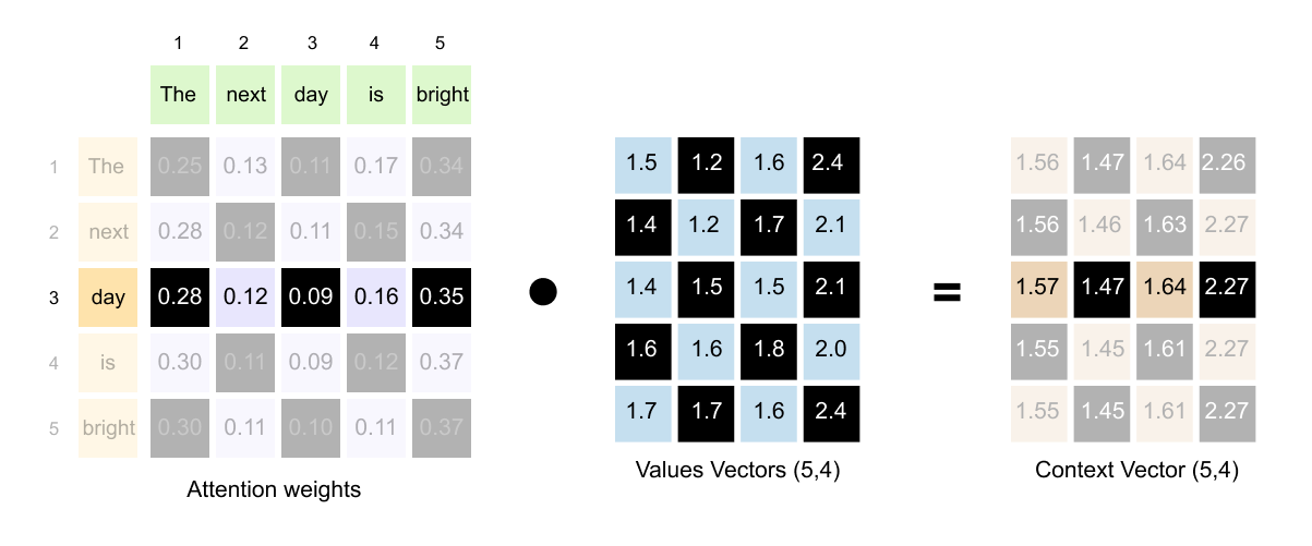
Figure 1.82: Computing the context vector for “day”: its attention weights are multiplied with the corresponding Value vectors and summed to produce a new representation that blends information from all tokens.
1. Get the Weights: We take row 3 from the Attention Weights matrix. These are the weights from “day” to all other tokens:
2. Get the Values: We use the entire (5, 4) Value matrix.
3. Perform the Weighted Sum: The new context vector for “day” is calculated by multiplying its attention weights by the corresponding Value vectors and summing the results:
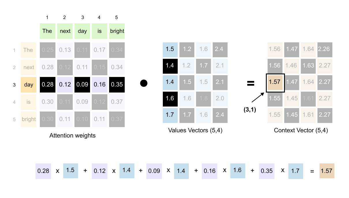
Figure 1.83: Detailed calculation showing how the first element of the context vector for “day” is computed as a weighted sum of the first elements of all Value vectors.
Since matrix calculations can sometimes feel overwhelming due to the number of values involved, You can see how how the value in the first column of the context vector for the token ‘day’ is calculated.
This new vector is a blend, or a weighted average, of all the tokens’ “value” representations. The blend is dictated by the attention scores. In this case, the new meaning of “day” is most heavily influenced by the value of “bright” (35%), followed by its own original value (9%), and the values of the other tokens.
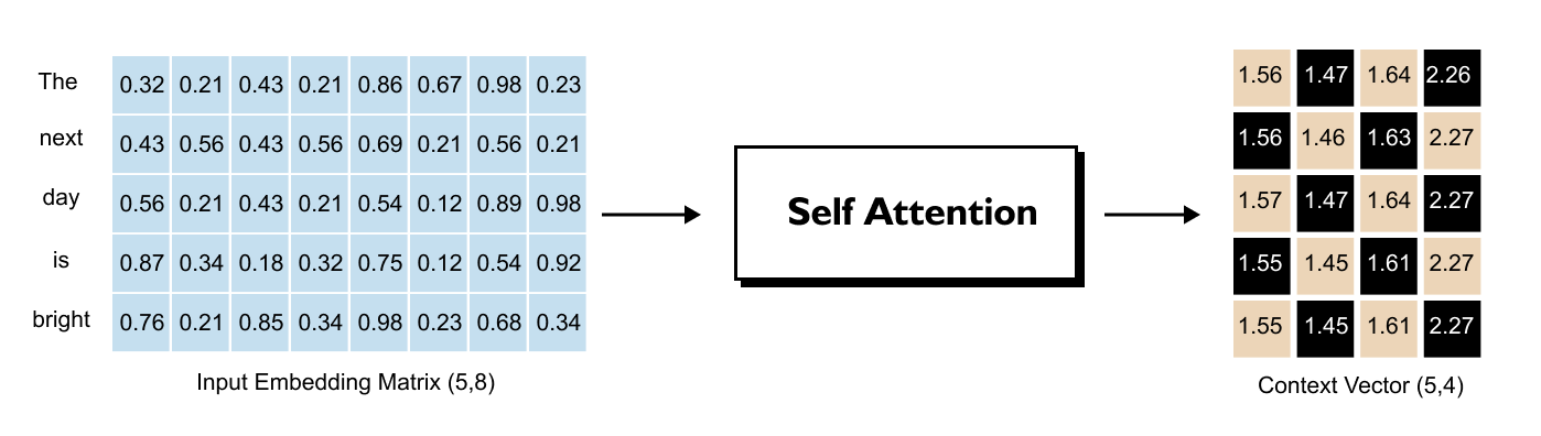
Figure 1.84 : The complete transformation: input embeddings (static, context-free) are converted into context vectors (dynamic, context-aware) through the self-attention mechanism.
We began with an input embedding matrix, where each token’s vector represented its meaning in isolation, unaware of its surroundings. The self-attention mechanism transforms these static inputs by projecting them into three new spaces: Query, Key, and Value. By comparing the Query and Key matrices, the model generates a matrix of attention weights. This weight matrix acts as a precise “blending recipe,” quantifying the exact relevance and relationship of every token to every other token in the sequence. The result is the context vector matrix, where each token’s original vector is replaced by a new, context-aware representation. This fundamental transformation from isolated, static meaning to a rich, contextualized representation is the central power of the self-attention mechanism.
Listing 1.7: Computing Context Vectors from Attention Weights
# compute context vectors for all tokens
context = attn_weights @ values      # shape (5, 4)

print(”Context vectors:”)
print(context)
print(”context.shape:”, context.shape)

# context vector for the word “next” only
context_next = attn_weights_next @ values
print(”\nContext vector for ‘next’:”)
print(context_next)
Output
Context vectors:
tensor([[ 2.2118,  2.4971, -0.2800,  0.8843],
        [ 2.2038,  2.4754, -0.2794,  0.8741],
        [ 2.2062,  2.4855, -0.2796,  0.8797],
        [ 2.2100,  2.4933, -0.2802,  0.8884],
        [ 2.2229,  2.5209, -0.2808,  0.9064]])
context.shape: torch.Size([5, 4])

Context vector for ‘next’:
tensor([ 2.2038,  2.4754, -0.2794,  0.8741])
The final step in self attention is to combine the value vectors using the attention weights as coefficients. Every context vector is a weighted sum of all value vectors, where the weights come from the corresponding row in the attention matrix.
The matrix product
context = attn_weights @ values
implements this operation for all five tokens at once. Since attn_weights has shape 5, 5 and values has shape 5, 4, the result has shape 5, 4. Each row in context is the new context aware representation of one token in the sentence.
The row context_next shows the updated representation for “next”. It lives in the same 4 dimensional space as the value vectors, but it now encodes information aggregated from all tokens in the sentence according to the learned attention pattern. This is exactly the transformation the theory section describes when it talks about going from static input embeddings to dynamic context vectors.
Listing 1.8: Packaging Self-Attention into a PyTorch Module
import torch.nn as nn

class SelfAttention(nn.Module):

    def __init__(self, d_in, d_out):
        super().__init__()
        self.W_query = nn.Parameter(torch.randn(d_in, d_out))
        self.W_key   = nn.Parameter(torch.randn(d_in, d_out))
        self.W_value = nn.Parameter(torch.randn(d_in, d_out))

    def forward(self, x):
        queries = x @ self.W_query    # (seq_len, d_out)
        keys    = x @ self.W_key      # (seq_len, d_out)
        values  = x @ self.W_value    # (seq_len, d_out)

        attn_scores  = queries @ keys.T
        d_k = keys.shape[-1]
        attn_weights = torch.softmax(
            attn_scores / d_k**0.5, dim=-1
        )

        context = attn_weights @ values
        return context

torch.manual_seed(123)
sa = SelfAttention(d_in=8, d_out=4)
out = sa(inputs)
print(out.shape)
output
torch.Size([5, 4])This class collects the individual steps of scaled dot product self attention into a reusable component. The constructor creates three trainable parameter matrices, each of shape d_in, d_out. When the module is part of a model, these parameters will be updated by the optimiser during training.
The forward method implements the same pipeline we derived by hand. It projects the input embeddings into queries, keys and values, computes all attention scores with a single matrix product, scales and normalises them with softmax, and finally uses the resulting weights to blend the value vectors into context vectors.
The last two lines create an instance of the layer with d_in equal to 8 and d_out equal to 4, apply it to the input sentence and print the shape of the output. The result 5, 4 confirms that for a sequence of five tokens the layer returns five context vectors, each living in the 4 dimensional space of the attention head. This is exactly the representation that will be passed on to the feed forward network in the transformer block.
1.13 Causal & Masked Attention
In the preceding section, we examined how self-attention transforms input embeddings into context-aware vectors. However, that explanation omitted a vital component for generative models: causal attention. This mechanism is fundamental, as it ensures that the model respects the sequential order of text and does not “cheat” by looking at future tokens.
Now that you have a solid understanding of the full self-attention pipeline, it is the perfect time to introduce this concept. This masking step is applied directly to the attention scores, just before the softmax function, to block any information from subsequent positions in the sequence.
Figure 1.85: Causal masking ensures that when processing token i, the model can only attend to tokens at positions 0 through i, preventing information leakage from future tokens.
Large language models like ChatGPT generate text by predicting one token at a time. Each predicted token is appended to the input, creating a growing context window used to predict the next token.
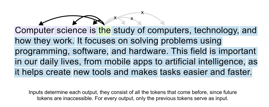
Figure 1.86: Sequential text generation: the model predicts one token at a time, appending each prediction to the input before generating the next.
This sequential process imposes a fundamental constraint: when computing the context vector for any token, only that token and preceding tokens should have influence. Future tokens must not contribute, as they have not yet been generated.
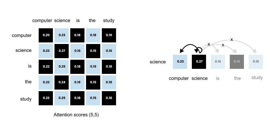
Figure 1.87 The causal constraint: when processing “science,” the model can only access “Computer” and itself. “is,” “the,” and subsequent tokens are masked out.
Consider the sequence “Computer” , “science”, “is” , “the”, “study...” When processing “science” , the model should only access itself and “Computer” . It must not see “is”, “the”, or any subsequent tokens. Similarly, “Computer” should only attend to itself, while “is” can attend to “Computer”, “science” , and itself, but not to the tokens that follow it.
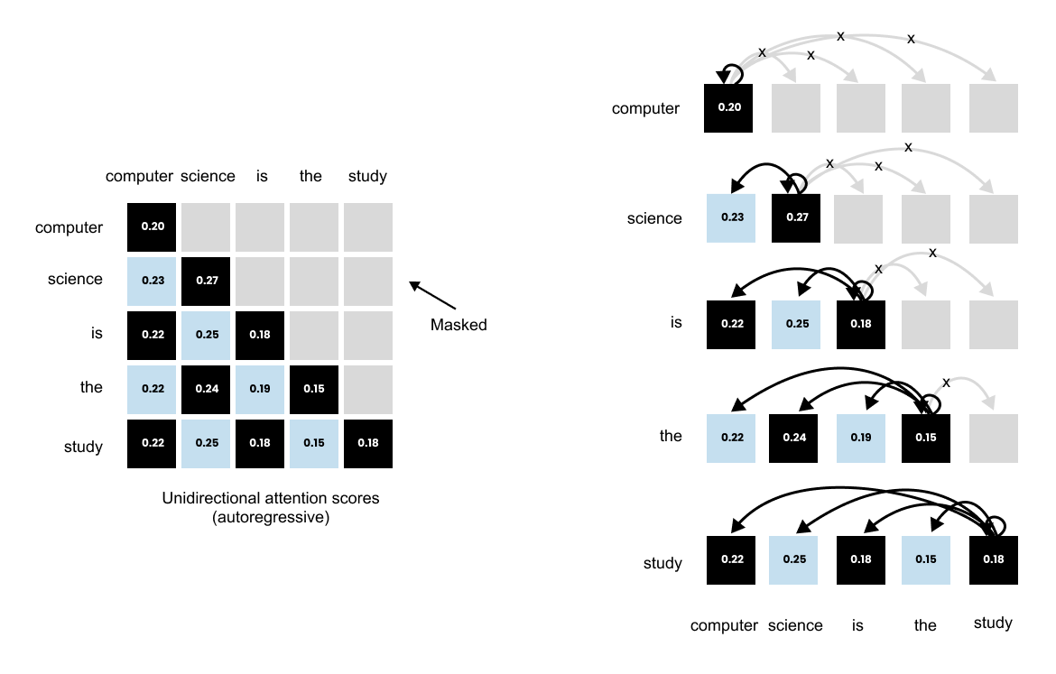
Figure 1.88: A lower-triangular attention matrix enforces the causal constraint. All entries above the diagonal are zero, ensuring that no token attends to future positions.
To enforce this constraint, we use masked attention. For each token acting as a query, we mask all keys corresponding to future positions by setting their attention scores to zero. The token “Computer” has a non-zero attention score only with itself. The token “science” has attention scores with “Computer” and itself, but zero scores with all future tokens like “is” and “the” . This masking creates a lower triangular attention matrix where all entries above the diagonal are zero.
After masking, we normalize the remaining attention weights in each row to sum to one. For “Computer” , the single remaining weight is set to one. For “science”, the two remaining weights are normalized so their sum equals one. This normalization is achieved by summing the non-masked weights in each row and dividing each weight by this sum, creating a proper probability distribution over the tokens each query can attend to. This mechanism, called causal attention or masked self attention, enables language models to generate coherent text while respecting the sequential nature of prediction.
Implementing Causal Attention through Zero Masking
To implement causal attention, we can begin with the raw attention scores. Consider the 5x5 attention score matrix for the sequence “computer science is the study”
Step 1: Initial Attention Scores
This is the raw, unnormalized matrix.
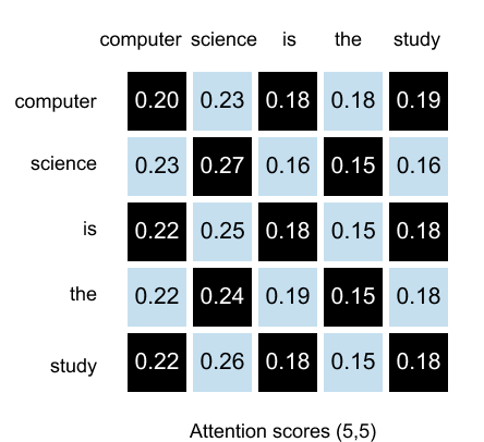
Figure 1.89: The raw 5×5 attention score matrix before any masking is applied.
In PyTorch, we can construct a lower triangular mask using the torch.tril()
torch.tril(MatrixA)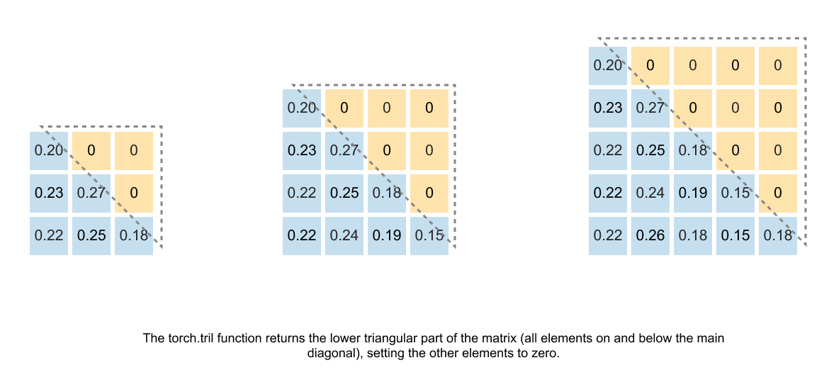
Figure 1.90: The torch.tril() function creates a lower-triangular mask: ones on and below the diagonal, zeros above.
This function creates a matrix where elements on and below the diagonal are ones, while elements above the diagonal are zeros. The size of this mask matrix must match the dimensions of our attention score matrix, which is determined by the context length.
The context length is simply the number of tokens currently in the sequence. For the example sequence “computer,” “science,” “is,” “the,” “study,” the context length is five.
Listing 1.9: Understanding Triangular Masks with torch.tril
import torch

# A simple 3x3 example matrix

A = torch.tensor([
    [1., 2., 3.],
    [4., 5., 6.],
    [7., 8., 9.],
])

print(”A:”)
print(A)

# Lower-triangular version of A

A_tril = torch.tril(A)

print(”\ntorch.tril(A):”)
print(A_tril)

# A pure mask built from ones

mask_ones = torch.tril(torch.ones_like(A))

print(”\nLower-triangular mask from ones:”)
print(mask_ones)

# Using the mask to zero out the upper triangle

A_masked = A * mask_ones

print(”\nA * mask_ones:”)
print(A_masked)
Output
A:
tensor([[1., 2., 3.],
        [4., 5., 6.],
        [7., 8., 9.]])

torch.tril(A):
tensor([[1., 0., 0.],
        [4., 5., 0.],
        [7., 8., 9.]])

Lower-triangular mask from ones:
tensor([[1., 1., 1.],
        [1., 1., 1.],
        [1., 1., 1.]]).tril()
tensor([[1., 0., 0.],
        [1., 1., 0.],
        [1., 1., 1.]])

A * mask_ones:
tensor([[1., 0., 0.],
        [4., 5., 0.],
        [7., 8., 9.]])
The function torch.tril returns the lower triangular part of a matrix: everything on and below the main diagonal is kept, everything above it is set to zero.
torch.tril(A) takes the original data in A and zeroes the entries above the diagonal.
torch.tril(torch.ones_like(A)) builds a mask: ones on and below the diagonal, zeros above.
Multiplying A by this mask with A * mask_ones keeps the lower triangle and zeroes out the upper triangle.
Causal attention uses exactly this idea. Instead of masking a 3×3 matrix, we mask a seq_len × seq_len attention score matrix so that token i can only see tokens 0..i and not future tokens.
Building a causal mask for a 5-token sequence
Assume we have a sequence of five tokens, such as:
[”computer”, “science”, “is”, “the”, “study”]
The attention scores attn_scores are a 5 x 5 matrix.
Listing 1.10: Building a Causal Mask for a 5-Token Sequence
seq_len = 5

# Build a 5x5 causal mask

causal_mask = torch.tril(torch.ones(seq_len, seq_len, dtype=torch.bool))

print(”Causal mask (True = allowed, False = masked):”)
print(causal_mask)
Output
Causal mask (True = allowed, False = masked):
tensor([[ True, False, False, False, False],
        [ True,  True, False, False, False],
        [ True,  True,  True, False, False],
        [ True,  True,  True,  True, False],
        [ True,  True,  True,  True,  True]])
This mask allows each token to only attend to itself and all previous tokens, blocking attention to future tokens to prevent information leakage.
Step 2: Create and Apply the Mask
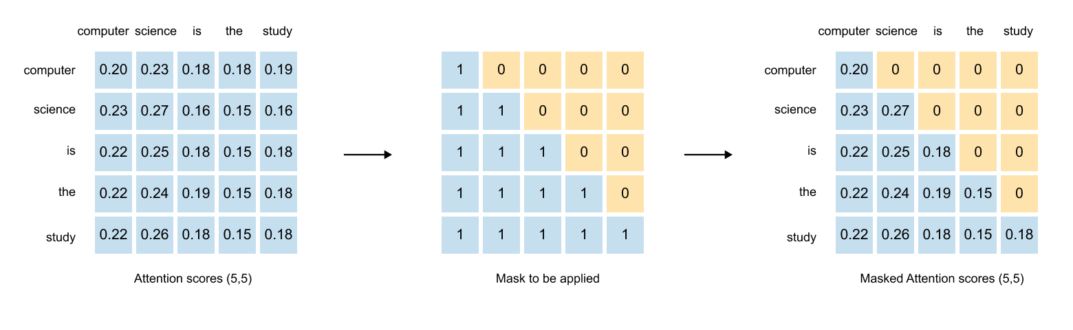
Figure 1.91: Applying the lower-triangular mask to the attention scores through element-wise multiplication zeros out all future-token entries.
The mask is created as a 5x5 lower triangular matrix of ones.
We then apply this mask to our attention scores through element-wise multiplication.
This operation sets all elements in the upper triangle to zero while preserving the lower triangular elements.
After multiplication, the attention scores that corresponded to future tokens are now zero, while scores for current and past tokens remain unchanged.
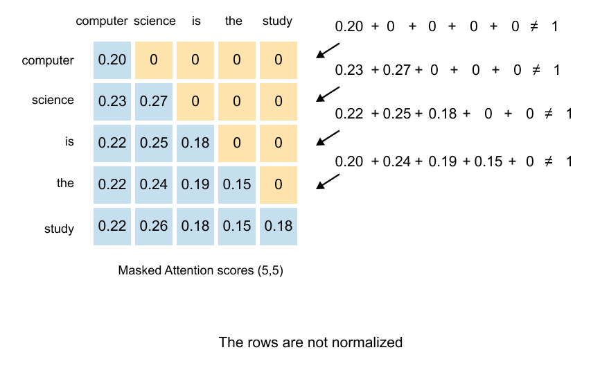
Figure 1.92: After masking, the rows are not yet normalized. Each row must be divided by its sum to form a valid probability distribution.
However, this masking alone is insufficient. The rows are not normalized and do not sum to one, which violates the requirement that attention weights form a probability distribution. We must normalize each row by dividing every element by the row sum, ensuring that the non-zero weights in each row sum to one.
Step 3: Row-wise Normalization
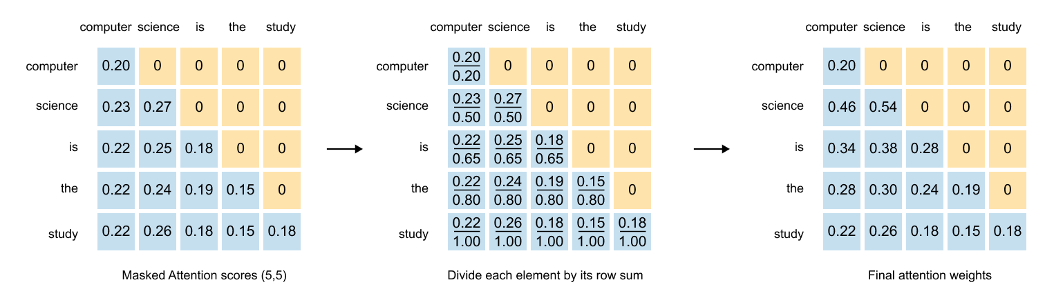
Figure 1.93: Row-wise normalization of the masked attention scores: dividing each entry by its row sum produces attention weights that sum to one.
First, we find the sum of each row in the masked matrix:
Now, we divide each element by its row sum to get the final weights.
This normalization step completes the implementation of this (flawed) version of causal attention.
The Problem: Data Leakage in Attention Computation
At first glance, the masked self-attention approach appears to solve the problem of preventing queries from attending to future tokens. We mask the upper triangular portion of the attention matrix and normalize the remaining weights. However, a closer examination reveals a critical flaw in this approach.
To understand the problem, we must revisit how attention weights are computed. The process begins with the construction of query, key, and value matrices. We compute the dot product between the query matrix and the transpose of the key matrix, producing attention scores that indicate how much each token attends to every other token. These scores are then scaled by dividing each element by the square root of the key dimensionality, yielding the scaled dot product. The crucial step occurs when we convert the scaled dot product into attention weights by applying the softmax function row-wise.
Here lies the problem. When we apply softmax to a row in the scaled dot product matrix, the denominator considers all elements in that row, including those corresponding to future tokens. Consider the first row, which corresponds to the token “computer.” When computing the softmax, the summation in the denominator includes the scaled dot product values for all tokens, including “science,” “is,” “the,” and “study.” Similarly, for the second row corresponding to “science,” the softmax denominator includes values from future tokens “is,” “the,” and “study.”
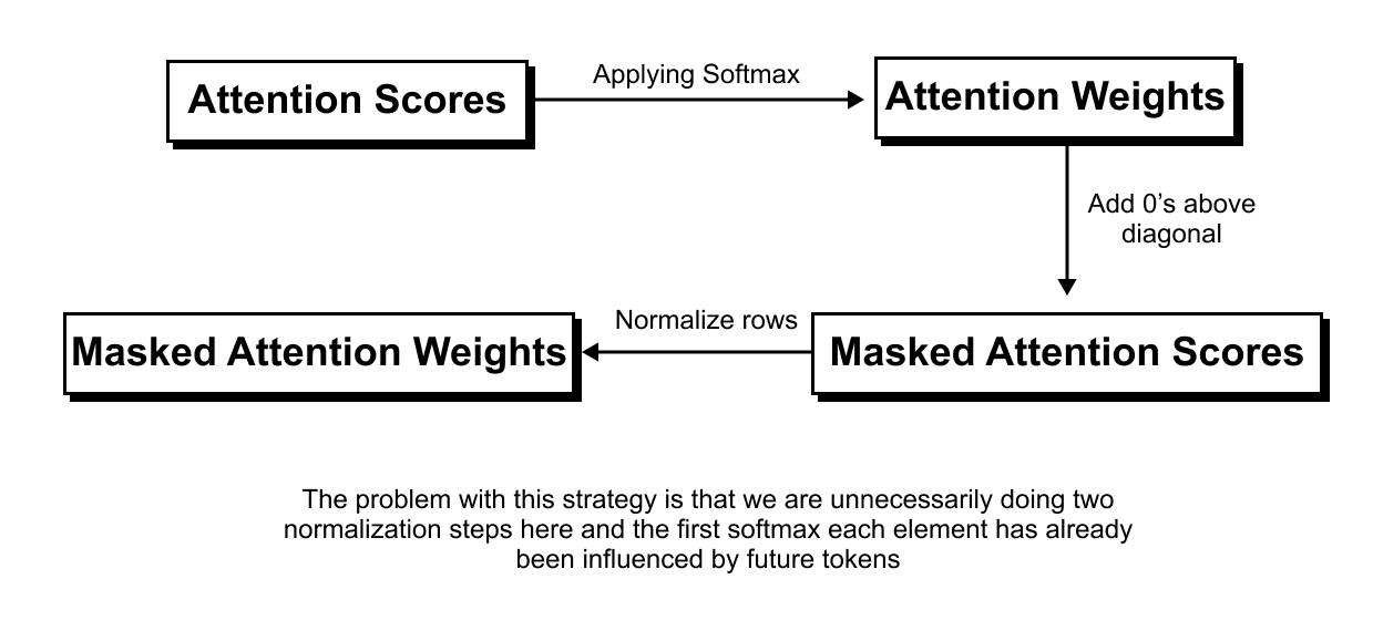
Figure 1.94: Data leakage: when softmax is computed before masking, the denominator already includes contributions from future tokens, subtly influencing the attention weights.
By the time we obtain the attention weights, each element has already been influenced by future tokens through the softmax normalization. Masking the attention weights after this computation does not eliminate this influence. The information from future tokens has already leaked into the computation through the softmax denominator.
This phenomenon is termed data leakage. We intended masked self-attention to prevent queries from accessing information about future tokens, but this prevention fails because the leakage occurs during the softmax computation itself.
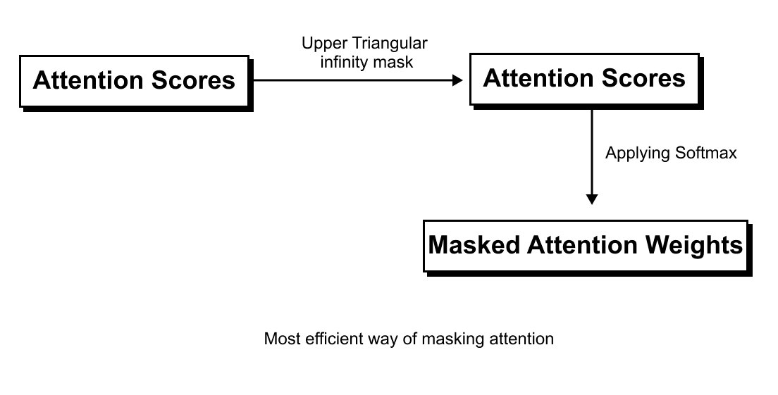
Figure 1.95: To prevent data leakage, masking must be applied before softmax so that future tokens are excluded from the softmax denominator entirely.
To properly implement causal attention, we must intervene before applying softmax. The softmax denominator for each row should only consider elements up to and including the current token position. Future keys must be excluded from this summation entirely. The masking operation must occur at the scaled dot product stage, before the softmax function is applied, to truly prevent data leakage.
The Solution: Masking with Negative Infinity
The solution to the data leakage problem involves a clever technique that applies masking before the softmax operation. Instead of zeroing out attention weights after computing softmax, we assign negative infinity values to the positions we want to mask in the scaled dot product matrix.
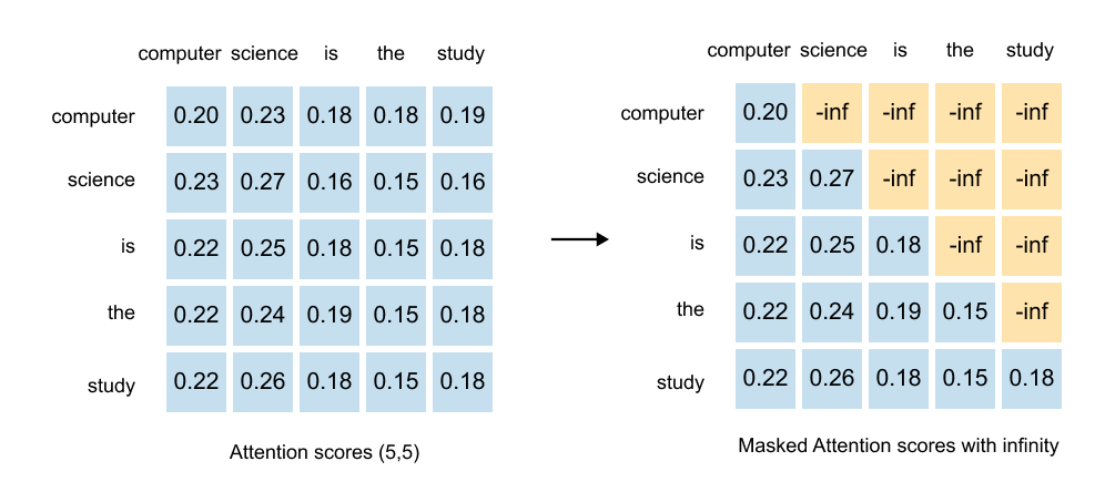
Figure 1.96: Negative infinity masking: upper-triangular entries are set to −∞ before softmax, which maps them to exactly zero probability while correctly normalizing over visible tokens.
The process works as follows. After computing the attention scores through the dot product between the query and key matrices, and before applying softmax, we set all upper triangular elements to negative infinity. These negative infinity values persist even after scaling by the square root of the key dimensionality, since dividing negative infinity by any finite number still yields negative infinity.
To understand why this approach works, consider how the softmax function behaves with negative infinity values.
Formula
Suppose we have a row containing the values 2, 3, and 5.
Then the values would be like below
Now consider what happens when we want to mask the last two elements. We replace them with negative infinity, giving us the sequence 2, negative infinity, negative infinity.
When we apply softmax, the first element is like this
The key insight is that
Therefore, the first element simplifies to 1
What happens to the masked elements?
Consider the second position containing negative infinity, it becomes zero. The third position similarly becomes zero as well.
After softmax, our sequence transforms into 1, 0, 0.
Let’s take one more example,
Now we are going to mask only the third element
The non-masked softmax values, 0.2689 and 0.7311, add up to one, which confirms they form a proper probability distribution over the unmasked elements
The elegance of this method lies in its automatic normalization property. By setting masked positions to negative infinity before softmax, the resulting attention weights naturally satisfy two requirements.
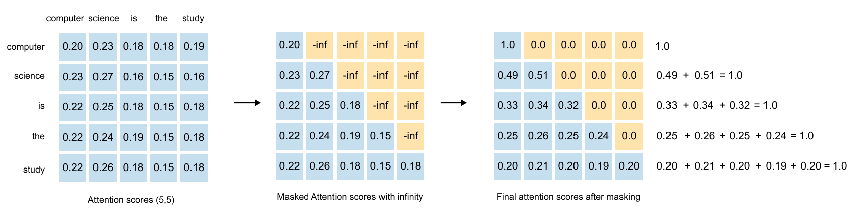
Figure 1.97: The complete causal masking pipeline: (1) compute scaled dot products, (2) set upper-triangular entries to −∞, (3) apply softmax. Masked positions become exactly zero with no data leakage.
First, all masked positions become exactly zero after softmax. Second, the remaining non-masked weights in each row automatically sum to one, as the softmax function guarantees normalization over all finite input values. This eliminates the need for any additional normalization step after masking, solving the data leakage problem while maintaining the mathematical properties required for attention weights.
Now we apply the causal mask to the scaled attention scores.
Listing 1.11: Applying the Causal Mask to Scaled Attention Scores
import math

scaled_scores = attn_scores / math.sqrt(d_k)
print(”Scaled scores (unmasked):”)
print(scaled_scores)

# Build the boolean causal mask again

seq_len = attn_scores.size(0)
causal_mask = torch.tril(torch.ones(seq_len, seq_len, dtype=torch.bool))

# Apply the mask: set disallowed positions to -inf

masked_scaled_scores = scaled_scores.masked_fill(~causal_mask, float(”-inf”))

print(”\nScaled scores with causal mask:”)
print(masked_scaled_scores)
Output
Scaled scores (unmasked):
tensor([[0.5000, 1.0000, 1.5000, 2.0000, 2.5000],
        [0.7500, 1.2500, 1.7500, 2.2500, 2.7500],
        [1.0000, 1.5000, 2.0000, 2.5000, 3.0000],
        [1.2500, 1.7500, 2.2500, 2.7500, 3.2500],
        [1.5000, 2.0000, 2.5000, 3.0000, 3.5000]])

Scaled scores with causal mask:
tensor([[0.5000,   -inf,   -inf,   -inf,   -inf],
        [0.7500, 1.2500,   -inf,   -inf,   -inf],
        [1.0000, 1.5000, 2.0000,   -inf,   -inf],
        [1.2500, 1.7500, 2.2500, 2.7500,   -inf],
        [1.5000, 2.0000, 2.5000, 3.0000, 3.5000]])
We first apply the usual scaling factor 1/sqrt(d_k) to the scores.
Then
masked_scaled_scores = scaled_scores.masked_fill(~causal_mask, float(”-inf”))does two things:
~causal_mask inverts the boolean mask. Positions that were False (future tokens) become True.
masked_fill writes -inf into those positions.
All allowed positions (on and below the diagonal) keep their original scaled scores. Disallowed positions become negative infinity. This guarantees that, when we apply softmax next, future tokens will contribute zero probability.
Now let’s apply softmax to make causal attention weights from masked scores
Listing 1.12: Computing Causal Attention Weights with Softmax
attn_weights_causal = torch.softmax(masked_scaled_scores, dim=-1)

print(”Causal attention weights:”)
print(attn_weights_causal)
print(”\nRow sums:”, attn_weights_causal.sum(dim=-1))
Output
Causal attention weights:
tensor([[1.0000, 0.0000, 0.0000, 0.0000, 0.0000],
        [0.3777, 0.6223, 0.0000, 0.0000, 0.0000],
        [0.1863, 0.3072, 0.5065, 0.0000, 0.0000],
        [0.1015, 0.1674, 0.2760, 0.4551, 0.0000],
        [0.0580, 0.0956, 0.1577, 0.2599, 0.4288]])

Row sums: tensor([1.0000, 1.0000, 1.0000, 1.0000, 1.0000])
Softmax is now applied to rows that contain finite scores only on and below the diagonal, while masked positions are set to −inf so their exponentials become zero. As a result, the first token can only attend to itself, giving a distribution like [1, 0, 0, 0, 0]; the second token attends only to the first two positions, and those two weights sum to one; the last token can attend to all five positions, so its row is a full probability distribution over the sequence. In every case, all entries above the diagonal are exactly zero, so no token ever attends to future tokens, and each row still sums to one, so every row is a valid attention distribution. Because this masking is applied before softmax, there is no data leakage from future positions, which gives us true causal attention.
1.14 Causal Attention with Dropouts
Concept of Dropout
Before exploring how dropout is applied in causal attention, we first review the concept of dropout and its purpose in neural networks. Dropout is a regularization technique designed to prevent overfitting and ensure that all neurons in a network contribute meaningfully to the learning process.
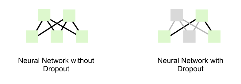
Figure 1.98: Dropout randomly deactivates neurons during training, forcing lazy neurons to participate and preventing the network from relying on a few dominant connections.
Consider a neural network layer where certain neurons dominate the computation while others contribute minimally. For example, in a layer with five neurons, one neuron might have very large weights while the other two have small weights. This dominant neuron effectively controls the output of the layer, while the other neurons become what we call lazy neurons. These lazy neurons do not significantly influence the forward pass and consequently do not learn useful representations during training. The network essentially overfits by relying too heavily on a subset of neurons.
Dropout addresses this problem by randomly deactivating neurons during training. In each forward pass through the network, neurons are switched off with a certain probability, typically 0.5. This means that statistically, half of the neurons will be deactivated in any given training iteration. The selection is probabilistic and automatic, not manual.
When a previously dominant neuron is switched off, the lazy neurons must participate in the forward propagation. During backpropagation, the weights of these previously inactive neurons must now be adjusted to minimize the loss. Without dropout, if the forward propagation relies entirely on one or two dominant neurons that already produce low loss, the weights of the lazy neurons would never be updated. By forcing different subsets of neurons to be active across training iterations, dropout ensures that all neurons learn to extract useful features from the data.
This technique prevents the network from becoming overly dependent on specific neurons and encourages the development of more robust, distributed representations across the entire network.
Why Dropout Matters in Attention Mechanisms
When we build attention mechanisms for language models, we sometimes encounter a problem where certain words become overly dependent on each other.
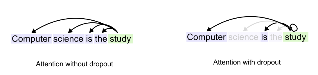
Figure 1.99: Without dropout, the word “study” may pay excessive attention to specific earlier words, memorizing patterns rather than learning general language rules.
Consider the sentence “computer science is the study.” If the word “study” pays excessive attention to specific earlier words, the model might memorize these particular patterns rather than learning general language rules. This excessive dependency between tokens can hurt the model’s ability to generalize to new sentences.
Dropout offers an elegant solution to this problem. By randomly removing some attention connections during training, we force the model to learn more robust patterns that don’t rely on any single strong connection.
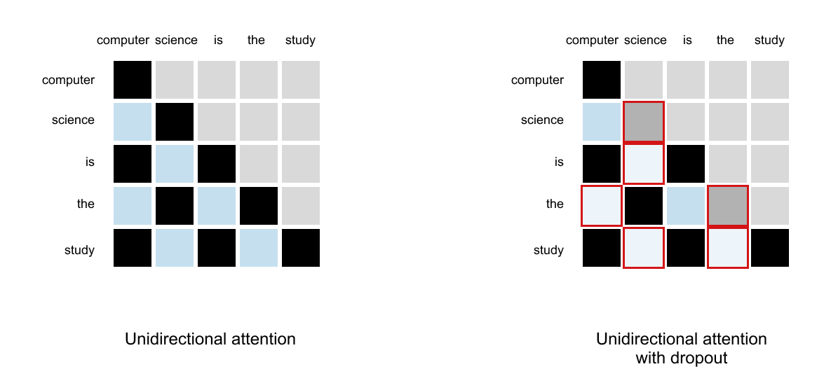
Figure 1.100: Causal attention with dropout applied: some valid attention connections (shown in red) are randomly zeroed out during training while the causal mask is preserved.
Let’s walk through where dropout fits in. Consider our example with 5 input tokens: “computer”, “science”, “is”, “the”, “study”. Each token gets represented as a vector, and as you have seen in the self attention section, we have Attention weights.
For unidirectional attention (also called causal attention), we mask the upper triangle of this matrix. This ensures that each token can only attend to previous tokens and itself, not future ones. Looking at the visualization, “computer” can only see itself , “science” can see “computer” and itself, “is” can see the first three words, and so on. The gray areas represent these masked positions where attention is blocked.
Here’s where dropout comes in. After obtaining the attention weights, we randomly set some of them to zero with probability p. In the right image, we see unidirectional attention with dropout applied. The red boxes highlight positions where dropout has been applied, effectively zeroing out those attention connections.
Notice how dropout respects the causal structure. It only affects the valid attention weights (the lower triangular part), never touching the already masked upper triangle. Some attention weights that were previously active are now dropped out (shown within red boxes), forcing the model to rely on different connection patterns.
The Scaling Factor Explained
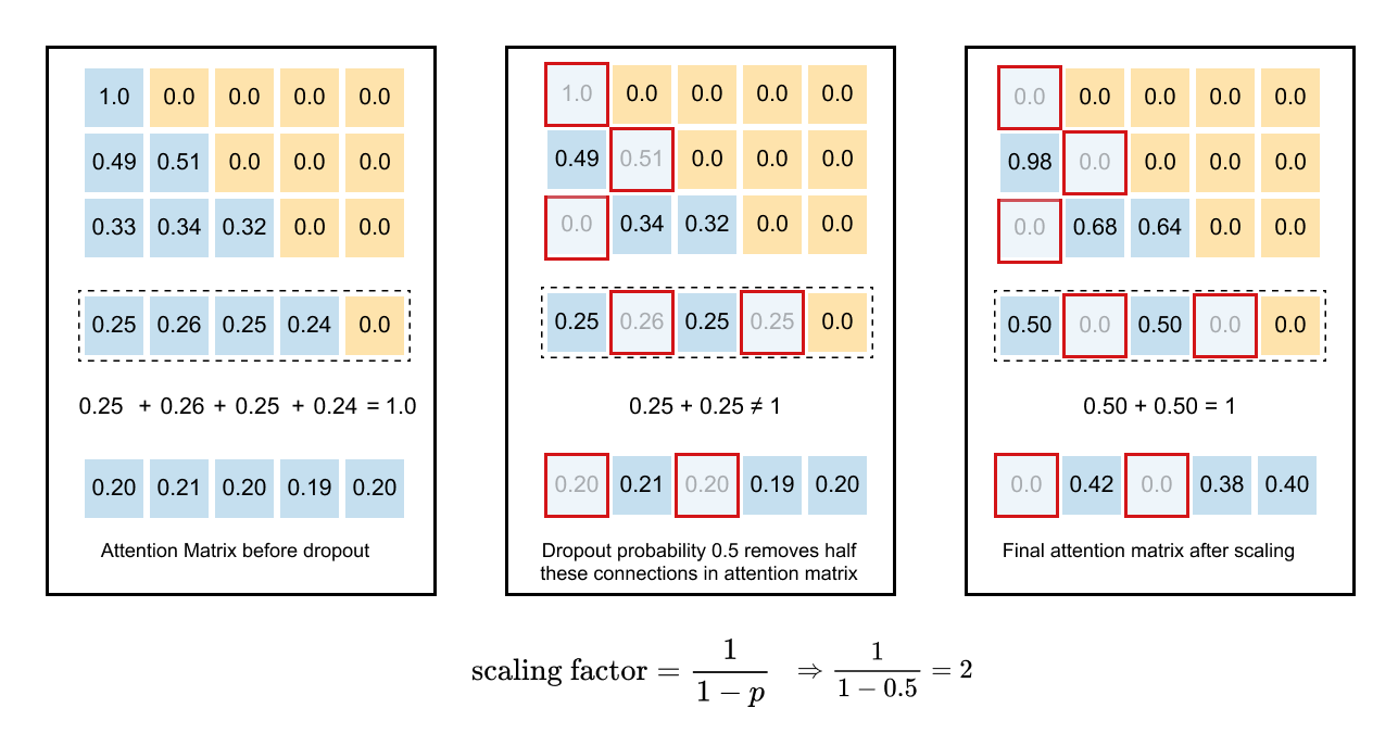
Figure 1.101: Dropout scaling: when connections are dropped with probability p, the remaining weights are scaled by 1/( 1−p) to maintain consistent expected output magnitude between training and inference.
When we apply dropout, there’s a crucial detail:
we need to scale up the remaining weights. This scaling maintains consistent behavior between training and inference. Suppose in row 4, we originally have attention weights distributed across the first four positions. If dropout with probability 0.5 removes half these connections, the remaining weights need to be doubled to maintain the same expected output magnitude. For example, referring to the matrix, if the fourth row originally had attention weights [0.25, 0.26, 0.25, 0.24] for its four non-zero positions, and dropout with probability 0.5 zeros out two of them, such as the second and fourth values, the remaining two might become [0.50, 0, 0.50, 0] after scaling by 2. This ensures the total signal strength remains consistent.
After applying dropout and scaling, each row of the attention matrix still represents a valid probability distribution over the tokens that can be attended to, just with fewer active connections.
This technique has become a standard component in transformer architectures, contributing to their remarkable success in natural language processing tasks. The simple act of randomly removing connections, combined with proper scaling, creates a powerful regularization effect that helps these models achieve better performance on unseen data.
Here let’s add dropout to the causal attention weights and then compute the context vectors.
We keep the same attn_weights_causal as above and assume we already have a values matrix of shape (5, 4) from the self-attention section.
Listing 1.13: Applying Dropout to Causal Attention Weights
dropout = torch.nn.Dropout(p=0.5)

torch.manual_seed(0)  # to get a stable example mask
attn_weights_causal_drop = dropout(attn_weights_causal)

print(”Causal attention weights before dropout:”)
print(attn_weights_causal)

print(”\nCausal attention weights after dropout (training mode):”)
print(attn_weights_causal_drop)
print(”Row sums after dropout:”, attn_weights_causal_drop.sum(dim=-1))

# Use the dropped weights to compute context vectors
context_causal = attn_weights_causal_drop @ values

print(”\nCausal context vectors with dropout:”)
print(context_causal)
print(”context_causal.shape:”, context_causal.shape)
Output
Causal attention weights before dropout:
tensor([[1.0000, 0.0000, 0.0000, 0.0000, 0.0000],
        [0.3777, 0.6223, 0.0000, 0.0000, 0.0000],
        [0.1863, 0.3072, 0.5065, 0.0000, 0.0000],
        [0.1015, 0.1674, 0.2760, 0.4551, 0.0000],
        [0.0580, 0.0956, 0.1577, 0.2599, 0.4288]])

Causal attention weights after dropout (training mode):
tensor([[2.0000, 0.0000, 0.0000, 0.0000, 0.0000],
        [0.7554, 0.0000, 0.0000, 0.0000, 0.0000],
        [0.3726, 0.6144, 0.0000, 0.0000, 0.0000],
        [0.2030, 0.3348, 0.0000, 0.9102, 0.0000],
        [0.0000, 0.1912, 0.3154, 0.5198, 0.0000]])

Row sums after dropout:
tensor([2.0000, 0.7554, 0.9870, 1.4480, 1.0264])

Causal context vectors with dropout:
tensor([[ 4.2400,  5.0200, -0.5600,  1.5400],
        [ 1.6020,  1.7000, -0.1600,  0.3700],
        [ 2.2640,  2.4060, -0.2700,  0.7000],
        [ 2.4240,  2.6460, -0.2800,  0.9700],
        [ 2.2670,  2.5410, -0.2800,  0.9100]])
context_causal.shape: torch.Size([5, 4])
Dropout randomly sets some attention weights to zero during training. Each weight is kept with probability 1 - p and dropped with probability p, and the remaining weights are scaled by 1 / 1 - p so that the expected total attention remains unchanged. Importantly, dropout never unblocks future positions, so all entries above the diagonal stay at zero and the causal structure is preserved. It only thins out the valid lower triangular connections. After this regularisation step, the dropped attention weights are still used in the usual way to compute the context vectors by multiplying them with the value matrix.
Finally, the context vectors are computed as
context_causal = attn_weights_causal_drop @ values
Each row of context_causal is the context vector for a token under causal attention with dropout. These vectors have shape (5,4), matching the number of tokens and the attention head dimension, and are what you feed into the feed-forward network inside a transformer block during training of generative models.
1.15 Summary of Self-Attention
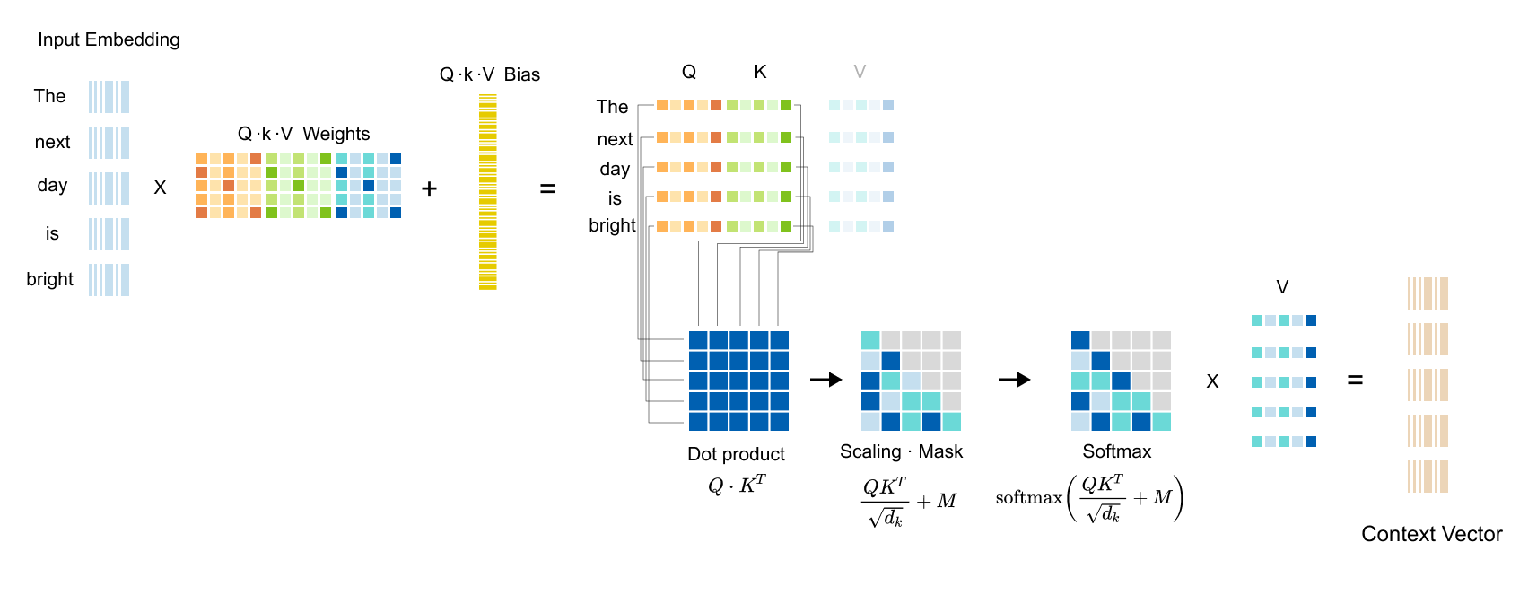
Figure 1.102: Complete self-attention pipeline: Input embeddings are projected into Q, K, V; attention scores are computed via QK^T , scaled, optionally masked, passed through softmax (with optional dropout), and multiplied by V to produce context vectors.
Before jumping into what multi-head attention is, let’s summarize the self-attention mechanism that we covered in the previous section. So the Process begins when the input tokens are converted into the Input Embedding matrix. This matrix is linearly projected into three distinct matrices: Query (Q), Key (K), and Value (V). This is achieved by multiplying the Input Embedding matrix by three separate, trainable weight matrices. Once Q, K, and V are generated, the input embedding matrix is no longer needed.
The core attention calculation starts by computing the Attention Scores. This is done, as shown in the first ‘MatMul’ step, by taking the dot product of the Q matrix with the transpose of the K matrix. These raw scores are then normalized in the ‘Scale’ step, where they are divided by the square root of the Key’s dimension. This scaling is crucial for stabilizing the gradients during training.
Following scaling, an ‘Optional Mask’ can be applied. This step is essential for implementing causal attention, where it masks out all scores corresponding to future tokens, ensuring a token can only attend to itself and previous tokens. Next, the SoftMax function is applied across each row of the scaled (and possibly masked) scores. This converts the scores into positive values that sum to one, effectively turning them into the final attention weights. An ‘Optional Dropout’ layer can be applied here to prevent overfitting.
In the final step, these attention weights are multiplied by the Value (V) matrix, as shown in the second ‘MatMul’ operation. This produces the Context Vector (Z). Each row of this Z matrix is a new, contextually enriched vector for the corresponding input token, as it now contains a weighted combination of information from all other tokens it was allowed to attend to.
Limitations of Self-Attention Mechanisms

Figure 1.103: Linguistic ambiguity: “The artist painted the portrait of a woman with a brush” has two valid interpretations, the brush is the tool for painting, or the woman in the portrait holds a brush.
A significant problem with a single self-attention mechanism is its limited ability to effectively handle linguistic ambiguity. This challenge can be illustrated with the sentence:
“The artist painted the portrait of a woman with a brush.”
This statement has two distinct and valid interpretations.
The first interpretation is that the artist used a brush as a tool to perform the action of painting. In this context, the phrase “with a brush” modifies the verb “painted”.
The second interpretation is that the subject of the painting is a woman who is holding a brush. Here, “with a brush” modifies the “woman” or “portrait”.
A single self-attention layer may struggle to capture both of these potential relationships simultaneously. It might incorrectly average these dependencies or fixate on only one, resulting in a contextual vector that fails to represent the full nuance of the sentence.
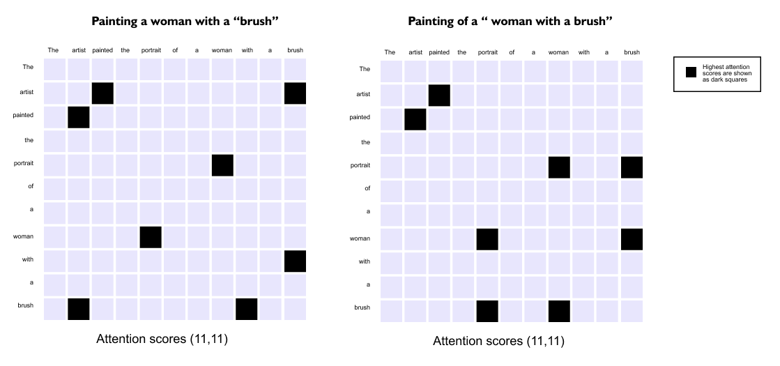
Figure 1.104: A single attention head can only produce one attention matrix, either capturing the tool interpretation or the subject interpretation, but not both simultaneously.
The first interpretation, where the artist uses the brush, would generate an attention score matrix where the word “artist” has a high attention score with “brush”.
The second interpretation, where the woman in the in the portrait is holding a brush, would generate a completely different matrix where “woman” and “portrait” have high attention scores with “brush”.
A single self-attention layer can only produce one of these attention matrices. It will either settle on one perspective or create an unhelpful average of the two. This results in a context vector that fails to represent the full richness and potential ambiguity of the input, limiting the model’s ability to understand the multiple angles or meanings present in complex language.
This limitation demonstrates the need for a more robust mechanism, which multi-head attention addresses.
1.16 Intuition of Multi-Head Attention
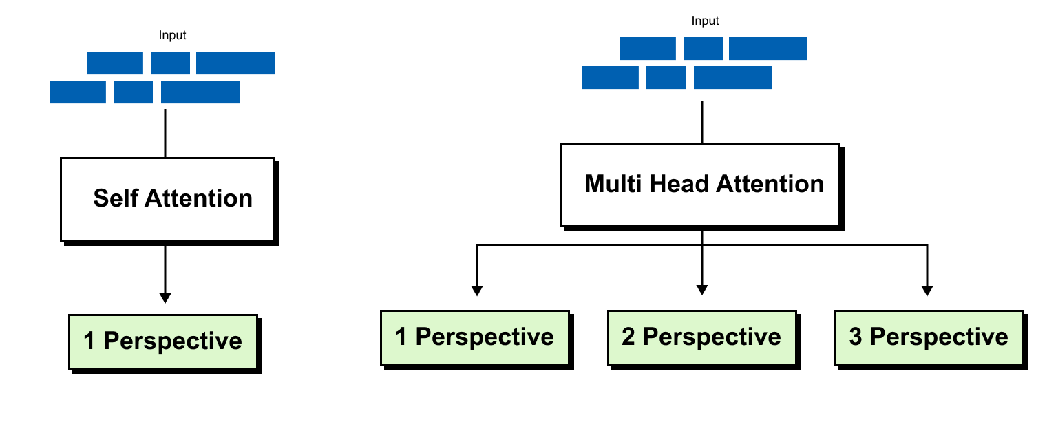
Figure 1.105: Multi-head attention: the same input is fed into multiple independent self-attention heads in parallel, each learning a different set of relationships. Their outputs are concatenated into a single enriched context matrix.
Since a single self-attention mechanism is limited to capturing only one perspective from an input sequence, the solution is to use multiple self-attention mechanisms in parallel. This architecture is known as multi-head attention. The core idea is that the same input embedding matrix is fed into several independent self-attention “heads”. Each head produces its own distinct context vector matrix, effectively learning a different set of relationships or focusing on a different aspect of the input, such as one head capturing verb-centric relationships while another captures a different semantic nuance. These individual context vector matrices, each representing a unique perspective, are then combined or merged. This process results in a single, final context vector matrix that is much richer, as it amalgamates the multiple perspectives captured by all the individual heads, leading to a more comprehensive representation of the input.
To implement multi-head attention, we must adapt the query, key, and value matrix operations to support multiple attention mechanisms operating in parallel. Having established the limitations of a single self-attention layer, the goal is to see how we can practically implement a system with multiple heads, for instance, a two-head attention mechanism. The procedure will demonstrate how to generate two independent sets of attention scores and two corresponding context vector matrices. This parallel processing is the core of multi-head attention, as it allows the model to produce multiple, distinct representations, with each head capturing a different perspective or set of relationships from the input sequence.
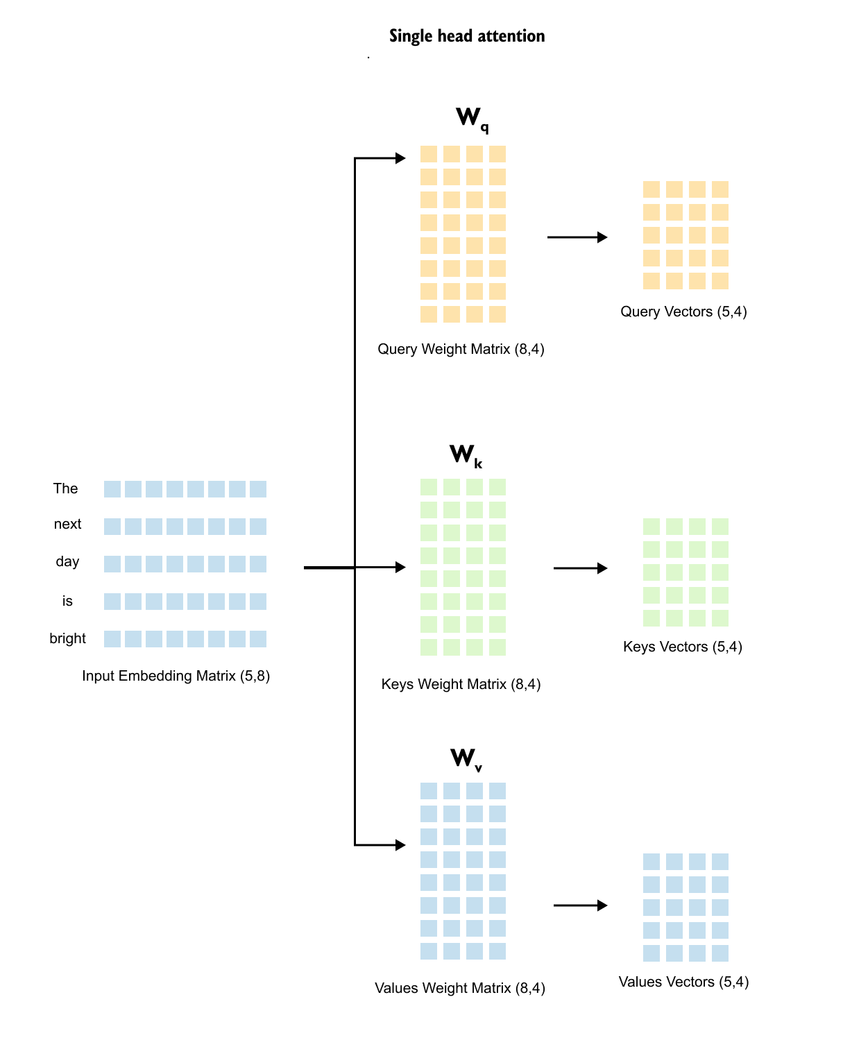
Figure 1.106: From single-head to two-head attention: the input embedding matrix is processed by separate weight matrices for each head, producing independent sets of Q, K, and V vectors.
The process begins with the input embedding matrix. Using the example sentence “The next day is bright”, which has 5 tokens, we start with an input embedding matrix. As illustrated, each token is represented by an embedding of eight dimensions. This configuration results in an input embedding matrix with dimensions of 5 by 8. The goal of a two head attention mechanism is to transform this single input matrix into two distinct context vector matrices, with each one capturing a different perspective.
To establish a baseline, recall the procedure for a single attention head. In this case, the 5 by 8 input embedding matrix is multiplied by three separate trainable weight matrices. As shown in the diagram, these are the Query Weight Matrix (W_q) with dimensions 8 by 4, the Keys Weight Matrix (W_k) with dimensions 8 by 4, and the Values Weight Matrix (W_v) with dimensions 8 by 4. This matrix multiplication operation produces a Query Vectors matrix (5 by 4), a Keys Vectors matrix (5 by 4), and a Values Vectors matrix (5 by 4). This single set of query, key, and value matrices is what the multi head attention mechanism will expand upon.
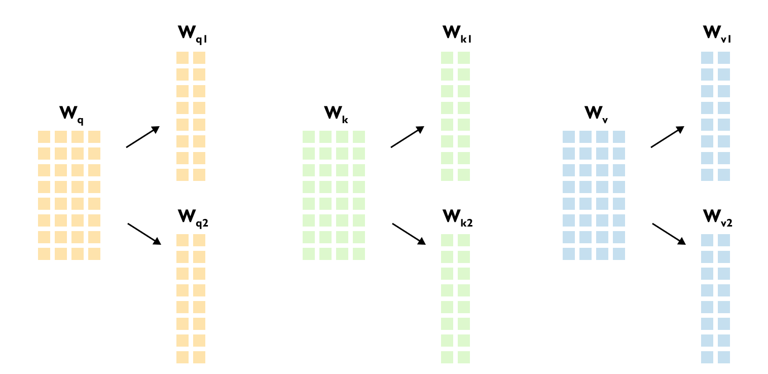
Figure 1.107: The head dimension: with d_out = 4 split across 2 heads, each head operates on a reduced dimension of 2. Weight matrices W_k1 and W_k2 each have shape (8, 2).
To transition from a single head to a multi head mechanism, such as one with two heads, the first step is to adapt the trainable weight matrices. Instead of one single query weight matrix (W_q), we now initialize two separate matrices, W_q1 and W_q2, one for each head. This same division is applied to the key and value matrices, creating W_k1, W_k2, W_v1, and W_v2}.
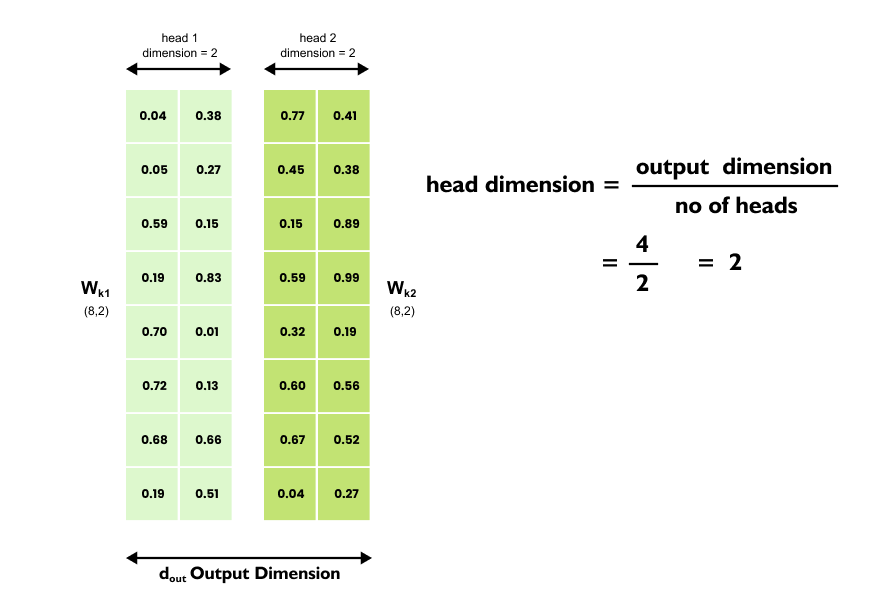
Figure 1.108: Each head operates on a reduced subspace. Head 1 produces Q1, K1, V1 of shape (5, 2); Head 2 produces Q2, K2, V2 of shape (5, 2).
The dimensions of these new matrices are determined by the “head dimension”. This value is calculated by dividing the original total output dimension (d_out) by the number of heads. For example, if the original d_out was 4, for a two head system, the head dimension is 4 divided by 2, which equals 2. This means that while the original weight matrices might have been 8 by 4, each new head specific matrix (like W_k1 and W_k2) will have dimensions of 8 by 2. The main idea of this step is to create multiple, smaller copies of the trainable W_q, W_k, and W_v matrices. As a direct consequence, this will naturally produce multiple sets of query vectors, key vectors, and value vectors when multiplied with the input embeddings.
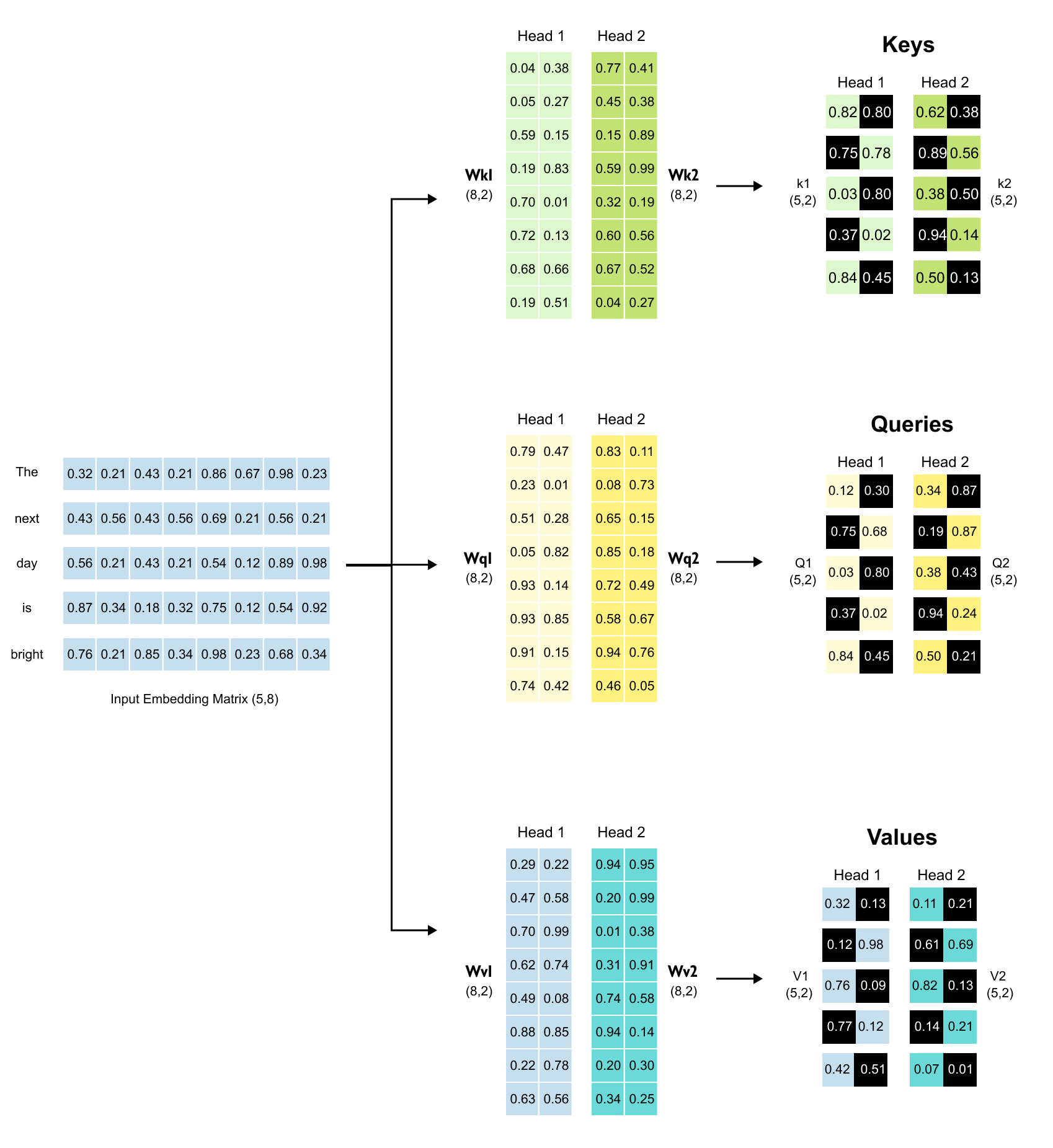
Figure 1.109: Parallel attention computation: the input embeddings are projected through head-specific weight matrices to produce independent Q, K, V matrices for each head
Multi-head attention extends the basic attention mechanism by creating parallel attention computations that can capture different types of relationships simultaneously. Starting with the input embedding matrix of dimensions 5×8 for our five tokens, the process splits attention into multiple heads. For a two-head configuration with output dimension of 4, each head operates on a reduced dimension of 2. The input embeddings are multiplied with separate weight matrices to produce Query, Key, and Value matrices for each head. Head 1 generates Q1, K1, and V1 matrices, while Head 2 produces Q2, K2, and V2 matrices, all with dimensions 5×2 to match the five tokens and head dimension of 2.
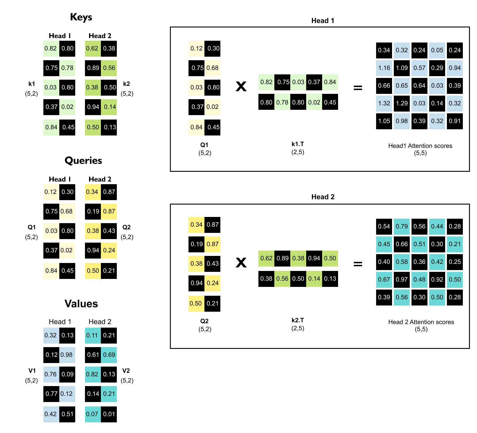
Figure 1.110: Each head independently computes its (5, 5) attention score matrix by multiplying Q with K^T , maintaining the ability to capture all pairwise token relationships.
Each head then independently computes its attention scores by multiplying its Query matrix with the transposed Key matrix.
The Query matrix for each head has shape (5,2) and the Key matrix has shape (2,5), where 5 represents the number of tokens in the sequence. When we multiply these matrices (Q times K transpose), we obtain a (5,5) attention score matrix for each head.
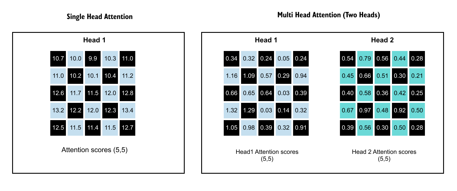
Figure 1.111: Two separate (5, 5) attention score matrices from two heads: each can capture different types of relationships in the data.
This is the crucial insight: although each head works with half the original dimension, the resulting attention score matrix maintains the full (5,5) shape, which represents relationships between all token pairs. This means that with 2 heads, we generate two separate (5,5) attention score matrices rather than one. Each matrix can capture different types of relationships in the data.
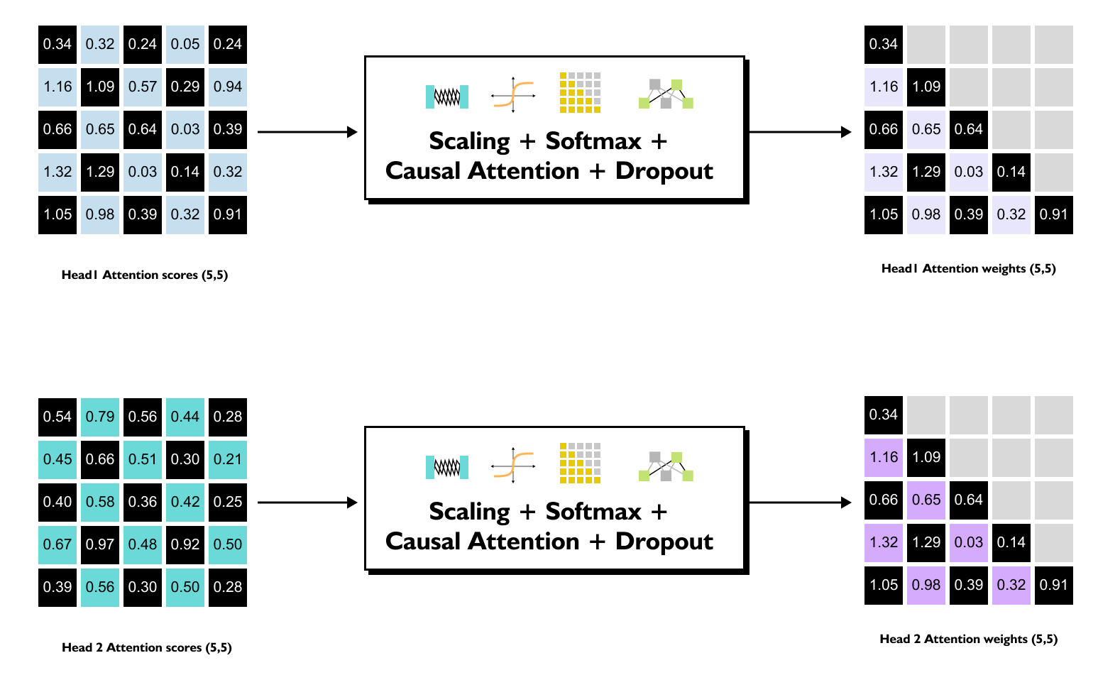
Figure 1.112: Each head independently applies scaling and softmax to produce its own attention weight matrix, then computes context vectors by multiplying with its Value matrix.
These attention scores then undergo the standard scaling and softmax normalization within each head independently. After computing the context vectors by multiplying the attention weights with the Value matrices, the outputs from all heads are concatenated back together to restore the original output dimension. This architecture allows the model to simultaneously learn and represent multiple perspectives of token relationships without increasing the computational cost compared to having a single attention mechanism with the full dimension.
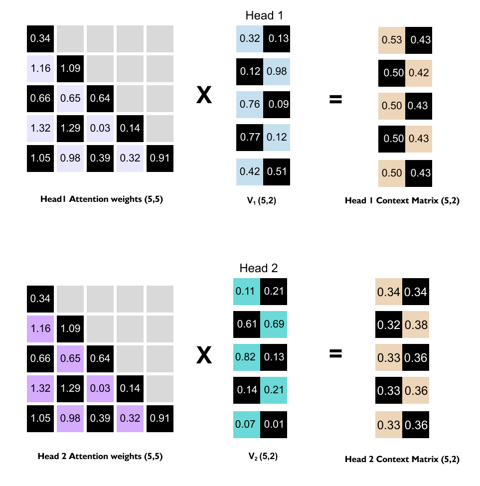
Figure 1.113: Context vectors from both heads: Head 1 produces a (5, 2) context matrix and Head 2 produces another (5, 2) context matrix, each capturing a different perspective.
Once we have the attention weight matrices for both heads, each of dimension, we proceed to compute the context vectors. This is done by multiplying each head’s attention weights with its corresponding Value matrix.
For Head 1, we multiply the (5,5) attention weight matrix with the (5,2) Value matrix V1, producing a (5,2) context matrix. Similarly, for Head 2, we multiply its (5,5) attention weight matrix with the (5,2) Value matrix V2, yielding another (5,2) context matrix. Each context matrix represents how the tokens should be represented based on the attention patterns learned by that particular head.
The final step in multi-head attention involves concatenating the context matrices from all heads to produce a unified output representation. Each head generates its own context matrix by multiplying its attention weights with its corresponding Value matrix.
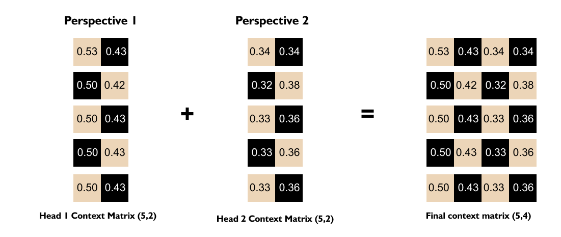
Figure 1.114: Concatenation: the (5, 2) outputs from Head 1 and Head 2 are concatenated along the feature dimension to recover the original output dimension, forming a (5, 4) final context matrix.
In our example with two heads processing a sequence of 5 tokens, Head 1 produces a context matrix representing the first perspective on token relationships, while Head 2 independently generates another context matrix capturing a second, distinct perspective. To combine these complementary perspectives, the context matrices are concatenated along the feature dimension. Specifically, the (5,2) matrix from Head 1 is placed alongside the (5,2) matrix from Head 2, forming a single (5,4) output matrix. This concatenation operation merges the outputs horizontally, stacking the feature vectors from each head side by side for every token position. The resulting (5,4) final context matrix maintains the sequence length of 5 tokens while recovering the original output dimension of 4, which equals the head dimension multiplied by the number of heads. This concatenated representation now contains the enriched information from both attention heads, allowing each token’s final representation to simultaneously encode multiple types of relationships and patterns discovered by the different heads. The concatenated output serves as the complete output of the multi-head attention mechanism and is typically passed through a final linear projection layer before proceeding to subsequent layers in the transformer architecture.
The Dimensional Trade-Off in Multi-Head Attention
While multi-head attention offers significant advantages in capturing diverse perspectives, it does involve a fundamental trade-off in its design. When the output dimension is split across multiple heads, each head operates with a reduced dimensionality compared to single-head attention. In our example with an output dimension of 4 split into 2 heads, each head works with only 2 dimensions rather than the full 4 dimensions that would be available in single-head attention. This reduction in per-head dimensionality means that each individual head has a smaller representational capacity and fewer parameters to capture nuanced patterns within its specific perspective. With fewer dimensions to work with, each head may be limited in the complexity and detail of the relationships it can encode. However, this apparent limitation is offset by the increased number of perspectives that can be learned in parallel. The architecture essentially implements a divide-and-conquer strategy: instead of attempting to capture all types of token relationships within a single high-dimensional space, the model distributes this learning task across multiple specialized heads, each focusing on different aspects of the input. While one head might capture syntactic dependencies with its 2 dimensions, another head simultaneously learns semantic relationships with its own 2 dimensions. This parallelization allows the model to explore a broader range of attention patterns across the same computational budget. The concatenation of outputs from all heads ultimately reconstructs the full output dimension, ensuring that the combined representation benefits from multiple complementary perspectives. Thus, while each head operates with reduced capacity, the overall multi-head architecture achieves greater expressiveness through diversification, making this trade-off worthwhile for most applications.
Listing 1.14: Creating the Input Tensor for Multi-Head Attention
import torch
torch.manual_seed(123)
torch.set_printoptions(precision=3, suppress=True)

# b, num_tokens, d_in = (1, 3, 6)
x = torch.tensor([[
    [1.0, 2.0, 3.0, 4.0, 5.0, 6.0],   # “The”
    [6.0, 5.0, 4.0, 3.0, 2.0, 1.0],   # “kid”
    [1.0, 1.0, 1.0, 1.0, 1.0, 1.0],   # “smiles”
]])

print(”x.shape:”, x.shape)
Output
x.shape: torch.Size([1, 3, 6])The tensor x holds one mini batch of token embeddings. The shape 1, 3, 6 reads as batch size one, three tokens per sequence, and six features per token. The three rows correspond to “The”, “kid”, and “smiles”, and each row has six embedding values.
Listing 1.15: Projecting Input to Query, Key, and Value
b, num_tokens, d_in = x.shape

d_out = 6          # final output dimension we want per token
num_heads = 2
head_dim = d_out // num_heads   # 6 // 2 = 3

W_q = torch.nn.Parameter(torch.randn(d_in, d_out), requires_grad=False)
W_k = torch.nn.Parameter(torch.randn(d_in, d_out), requires_grad=False)
W_v = torch.nn.Parameter(torch.randn(d_in, d_out), requires_grad=False)

q = x @ W_q    # (1, 3, 6)
k = x @ W_k    # (1, 3, 6)
v = x @ W_v    # (1, 3, 6)

print(”q.shape:”, q.shape)
print(”k.shape:”, k.shape)
print(”v.shape:”, v.shape)
Output
q.shape: torch.Size([1, 3, 6])
k.shape: torch.Size([1, 3, 6])
v.shape: torch.Size([1, 3, 6])
Instead of having separate weight matrices for each head, we follow the weight splitting idea. We keep a single large query, key, and value matrix of shape 6, 6 Multiplying the 1, 3, 6 input by a 6, 6 weight gives new 1, 3, 6 tensors for q, k, and v. At this point there is no explicit notion of heads in the tensors; all six output features per token are packed into the last dimension.
Listing 1.16: Splitting Projections into Multiple Heads
# reshape from (b, num_tokens, d_out) to (b, num_tokens, num_heads, head_dim)
q = q.view(b, num_tokens, num_heads, head_dim)
k = k.view(b, num_tokens, num_heads, head_dim)
v = v.view(b, num_tokens, num_heads, head_dim)

print(”q after view:”, q.shape)
print(”k after view:”, k.shape)
print(”v after view:”, v.shape)
Output
q after view: torch.Size([1, 3, 2, 3])
k after view: torch.Size([1, 3, 2, 3])
v after view: torch.Size([1, 3, 2, 3])
The six features that came out of each projection are now interpreted as two heads with three features each. The view operation does not change any values; it only changes how we index them. The new shape 1, 3, 2, 3 can be read as batch size one, three tokens, two heads, three features per head. For a given token position, the last two dimensions now contain the representation for head one and head two.
Listing 1.17: Reordering Dimensions to Group by Head
# move the head dimension in front of the token dimension
# from (b, num_tokens, num_heads, head_dim)
# to   (b, num_heads, num_tokens, head_dim)
q = q.transpose(1, 2)
k = k.transpose(1, 2)
v = v.transpose(1, 2)

print(”q after transpose:”, q.shape)
print(”k after transpose:”, k.shape)
print(”v after transpose:”, v.shape)
Output
q after transpose: torch.Size([1, 2, 3, 3])
k after transpose: torch.Size([1, 2, 3, 3])
v after transpose: torch.Size([1, 2, 3, 3])
After splitting into heads, it is convenient to group all tokens that belong to the same head together. The transpose call swaps the token and head axes. The new shape 1, 2, 3, 3 reads as batch size one, two heads, three tokens, three features per head. If you isolate q[0, 0] you see the three query vectors for head one, while q[0, 1] contains the three query vectors for head two. The same interpretation holds for k and v. This layout allows a single tensor operation to compute attention for all heads in parallel.
Listing 1.18: Computing Per-Head Attention Scores and Context Vectors
import math

# scaled dot product attention for all heads at once
scores = q @ k.transpose(-1, -2)        # (b, num_heads, num_tokens, num_tokens)
print(”scores.shape:”, scores.shape)

scale = math.sqrt(head_dim)
weights = torch.softmax(scores / scale, dim=-1)
print(”weights.shape:”, weights.shape)
print(”weights[0, 0]:”)
print(weights[0, 0])

# context vectors inside each head
context = weights @ v                   # (b, num_heads, num_tokens, head_dim)
print(”context per head shape:”, context.shape)
print(”context[0, 0]:”)
print(context[0, 0])
Output
scores.shape: torch.Size([1, 2, 3, 3])
weights.shape: torch.Size([1, 2, 3, 3])
weights[0, 0]:
tensor([[0.59 , 0.24 , 0.17 ],
        [0.29 , 0.45 , 0.26 ],
        [0.22 , 0.31 , 0.47 ]])
context per head shape: torch.Size([1, 2, 3, 3])
context[0, 0]:
tensor([[ 0.564, -3.817,  2.064],
        [ 3.116,  9.936, 14.649],
        [-2.124, -4.104,  2.056]])
The tensor scores has shape 1, 2, 3, 3. For each batch and head, it contains a full three by three attention score matrix over the three tokens. Dividing by sqrt(head_dim) and applying softmax along the last axis converts these scores into attention weights, again separately for each head. The shape of weights matches that of scores.
Multiplying the weights by v produces the context tensor of shape 1, 2, 3, 3. For each head you now have three context vectors, one per token, each with three features. In the printed slice context[0,0] you can see the three vectors produced by the first head for “The”, “kid”, and “smiles”, which match the output structure.
Listing 1.19: Merging Heads into the Final Context Matrix
# move tokens back in front of heads and merge head and feature dimensions
context = context.transpose(1, 2).contiguous()  # (b, num_tokens, num_heads, head_dim)
context = context.view(b, num_tokens, num_heads * head_dim)

print(”final context.shape:”, context.shape)
print(”final context:”)
print(context)
Output
final context.shape: torch.Size([1, 3, 6])
final context:
tensor([[[ 0.564, -3.817,  2.064,  3.116,  9.936, 14.649],
         [-2.124, -4.104,  2.056,  3.098,  9.814, 14.479],
         [-2.120, -4.099,  2.053,  3.113,  9.915, 14.620]]])
To return to a single context matrix per token, we undo the earlier reordering and then collapse the head dimension and the per head feature dimension back into one. The transpose moves us from 1, 2, 3, 3 to 1, 3, 2, 3 grouping all heads for each token together. The final view then interprets the last two dimensions 2, 3 as a single dimension of size six.
The result is a 1, 3, 6 tensor. Each row is now a six dimensional context vector for one token, built by concatenating the three features from head one and the three features from head two. Compared to single head attention, nothing about the scoring or weighting changed. The difference is that we used reshaping and transposing to let two separate attention heads operate in parallel on smaller subspaces, then merged their outputs to recover the original six dimensional representation per token.
Concluding Multi Head Attention
Multi head attention extends single head attention by running several independent attention mechanisms in parallel, each with its own learned query, key, and value projections on a reduced head dimension. For an input embedding matrix, each head produces its own attention scores over all token pairs and then its own context matrix, so different heads can specialize on different types of relationships in the sequence. These context matrices are then concatenated along the feature dimension to recover the original output size, so each token representation combines multiple complementary views of the same input. While each head has fewer dimensions and therefore lower capacity than a single large attention module, the collection of diverse heads makes the overall representation more expressive, and a final linear projection can further mix and refine these combined features.
1.17 Layer Normalization
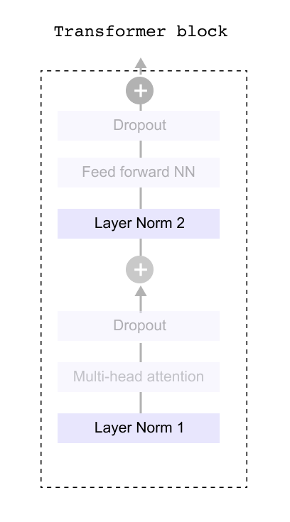
Figure 1.115: Layer normalization appears multiple times in the transformer block: before multi-head attention, before the feed-forward network, and often before the output layer.
In the transformer block, layer normalization appears several times. It is applied before the multi head attention sublayer, again before the feed forward network, and often once more outside the block before the final output layer. Because it is used so frequently, it is convenient to implement it as its own reusable module when we code the model.
Figure 1.116: The gradient flow problem in deep networks: without normalization, gradients can explode (very large activations) or vanish (very small activations), making training unstable.
To understand why layer normalization is so important, it helps to step back and look at a standard deep neural network with an input layer, several hidden layers, and an output layer. During the forward pass, activations flow from left to right, and during backpropagation the gradients flow in the opposite direction, from the output layer back through each hidden layer to the input.
Each layer has parameters and therefore receives gradients of the loss with respect to those parameters. The gradients at a given layer depend strongly on the outputs of that layer. If the layer outputs are very large in magnitude, the corresponding gradients tend to become very large as we chain them backward through the network. By the time they reach the earlier layers, they can explode to extremely large values. This is the exploding gradient problem and it leads to unstable updates and divergence during training.
The opposite can also happen. If the outputs of a layer are very small, the gradients that depend on them can quickly shrink as they propagate backward through many layers. Early layers then receive gradients that are almost zero and their parameters barely change. This is the vanishing gradient problem and it makes learning extremely slow or stops it altogether.
In both cases, very large or very small activations in intermediate layers create gradient magnitudes that are either too large or too small. Training then becomes unstable and inefficient. One way to stabilize the gradients is therefore to control the magnitude of the layer outputs themselves. This is exactly what normalization layers are designed to do.
Internal covariate shift
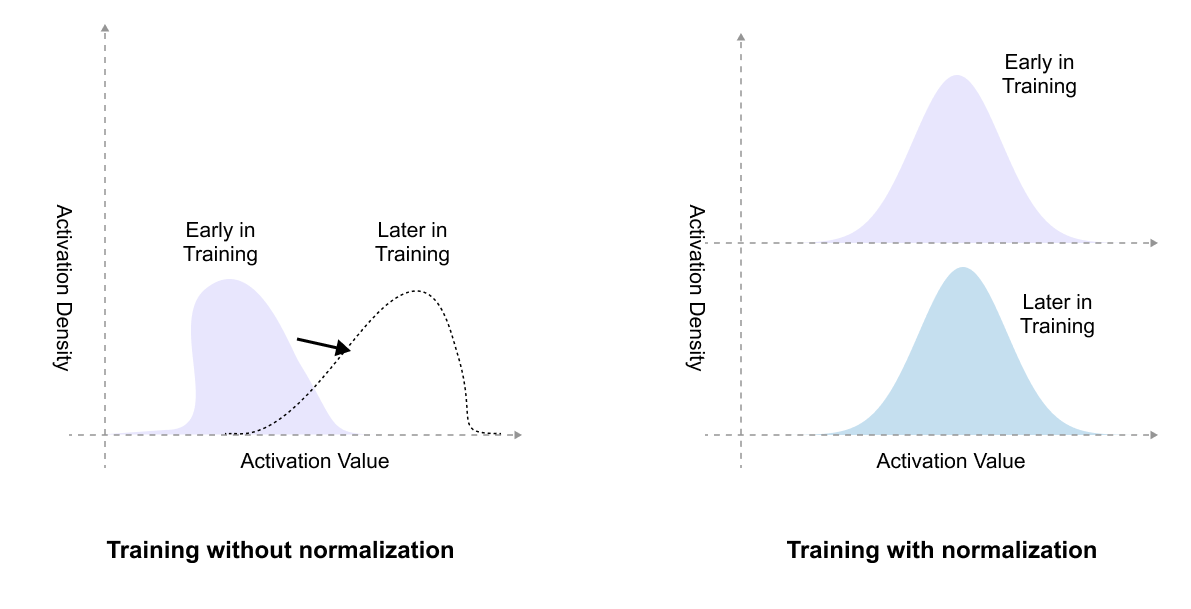
Figure 1.117: Internal covariate shift: as earlier layers update their weights during training, the distribution of activations fed into later layers keeps changing, making learning a moving target.
There is a second issue in deep networks known as internal covariate shift. During training, as earlier layers update their weights, the distribution of activations that they feed into later layers keeps changing. Imagine looking at the inputs to a particular hidden layer at the beginning of training. They may roughly follow one distribution. After a few training iterations, as weights update, the same layer may now see inputs with a different mean or variance, or a skewed shape. The layer is trying to learn a good mapping, but the distribution of its inputs keeps drifting, so the layer is constantly adapting to a moving target. This slows down convergence and makes optimization harder.
If we could keep the mean and variance of the inputs to each layer more stable across training iterations, learning would become easier. Normalization does this by rescaling activations so that their distribution is more consistent over time. This reduces internal covariate shift and helps the model converge faster.
The core idea of layer normalization
Layer normalization is a simple procedure applied to the outputs of a layer. Consider a single training example and focus on the vector of activations produced by some layer for that example.
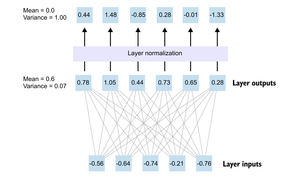
Figure 1.118: Layer normalization in action: six activations with mean 0.6 and variance 0.07 are centered to mean 0 and rescaled to variance 1, producing standardized activations.
Imagine a single layer that produces six outputs for one training example
These are the values shown in the middle row of the figure. Layer normalization first computes the mean of these activations
Next it computes the variance
When each activation xi is normalized, it is first shifted so its mean becomes zero, and then it is rescaled so its variance becomes one. This process is known as centering and rescaling. The formula
means that for each output value, you subtract the average of all outputs (centering), and then divide by their standard deviation (rescaling). This transformation ensures that the set of normalized activations has an average of zero and a unit variance, making them easier for the next layer of a neural network to process.
If you perform this computation for all six values, you obtain approximately
These are the normalized outputs shown in the top row of the figure. By construction, the mean of these normalized activations is zero and their variance is one, which is why the left side of the illustration reports mean equal to 0.0 and variance equal to 1.00. This example demonstrates how layer normalization transforms a set of layer outputs with mean 0.6 and variance 0.07 into a standardized set of activations that are better behaved numerically, making gradient based training more stable.
In practice, layer normalization is usually followed by a learned scale and shift. After computing the normalized activations x hat i, the layer produces new activations
Here gamma and beta are trainable parameters with the same size as the activation vector. They let the model undo or modify the standardization whenever that helps performance. In other words, the network can learn whatever output distribution it prefers, while still enjoying the stabilizing effect of normalization during training.
The way mean and variance are computed is what distinguishes layer normalization from batch based methods. For layer normalization we normalize across the features of a single example, not across different examples in a mini batch. Each token representation or layer output vector is treated independently and normalized across its dimensions. This makes the procedure independent of batch size and very convenient for transformer models that see variable length sequences and perform autoregressive decoding one token at a time.
Inside a transformer block, layer normalization is applied to the token representations before they enter the multi head attention module. This keeps the scale of the inputs to attention under control and stabilizes its gradients. After attention and its residual shortcut, layer normalization is applied again before the feed forward network so that this network also sees well behaved activations. Many architectures further normalize the final outputs of each block, and often the outputs of the last block before the language modeling head that predicts the next token.
1.18 FeedForward Network
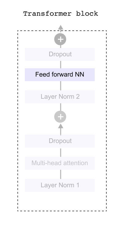
Figure 1.119: The feed-forward network sits between dropout and layer normalization inside each transformer block, processing each token representation independently
The second major component inside a transformer block, after the multi head attention, is the feed forward network. In the block diagram this appears as the Feed forward NN box, sitting between dropout and layer normalization. Conceptually it is an ordinary two layer neural network with an activation function in the middle, applied independently to every token representation. The key is that the same small network, with the same weights, is reused for all tokens and all examples in the batch.
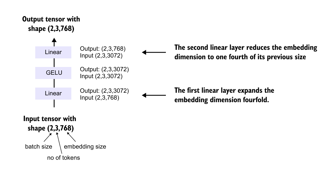
Figure 1.120: The feed-forward network processes each token vector independently using shared weights. For an input tensor of shape (batch, tokens, 768), each 768- dimensional vector is processed in parallel.
2, 3, 768. The first entry is the batch size, the second is the number of tokens in the context window, and the third is the embedding dimension for each token. The important point is that the feed forward network is applied to every token vector of length 768 independently but it uses the same weights for all tokens and all examples in the batch.
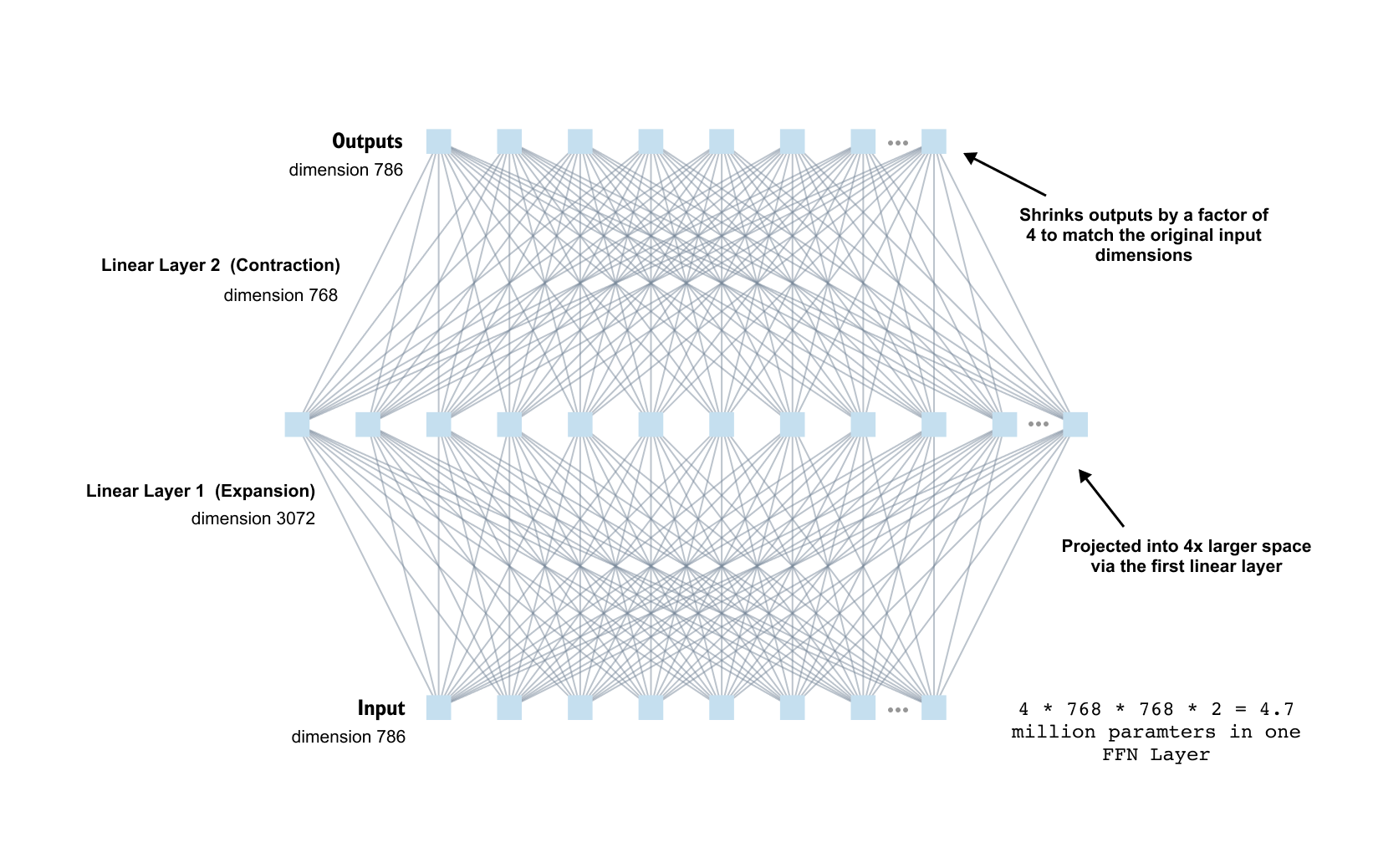
Figure 1.121: Internal structure of the feed-forward network: a linear expansion from 768 to 3072 dimensions, followed by GELU activation, then linear contraction back to 768 dimensions.
The internal structure of this network is shown in the detailed diagrams. It consists of two linear layers with an activation function in between. The first linear layer performs an expansion. It takes each 768 dimensional input vector and projects it into a much larger space with 4 × 768 = 3072 hidden units. In matrix form this is a multiplication by a 768 by 3072 weight matrix plus a bias term. Intuitively, this expansion gives the model more capacity to construct rich intermediate features from each token representation before compressing them again. Because every input dimension interacts with every hidden unit, this single layer already introduces dense mixing among the 768 input features.
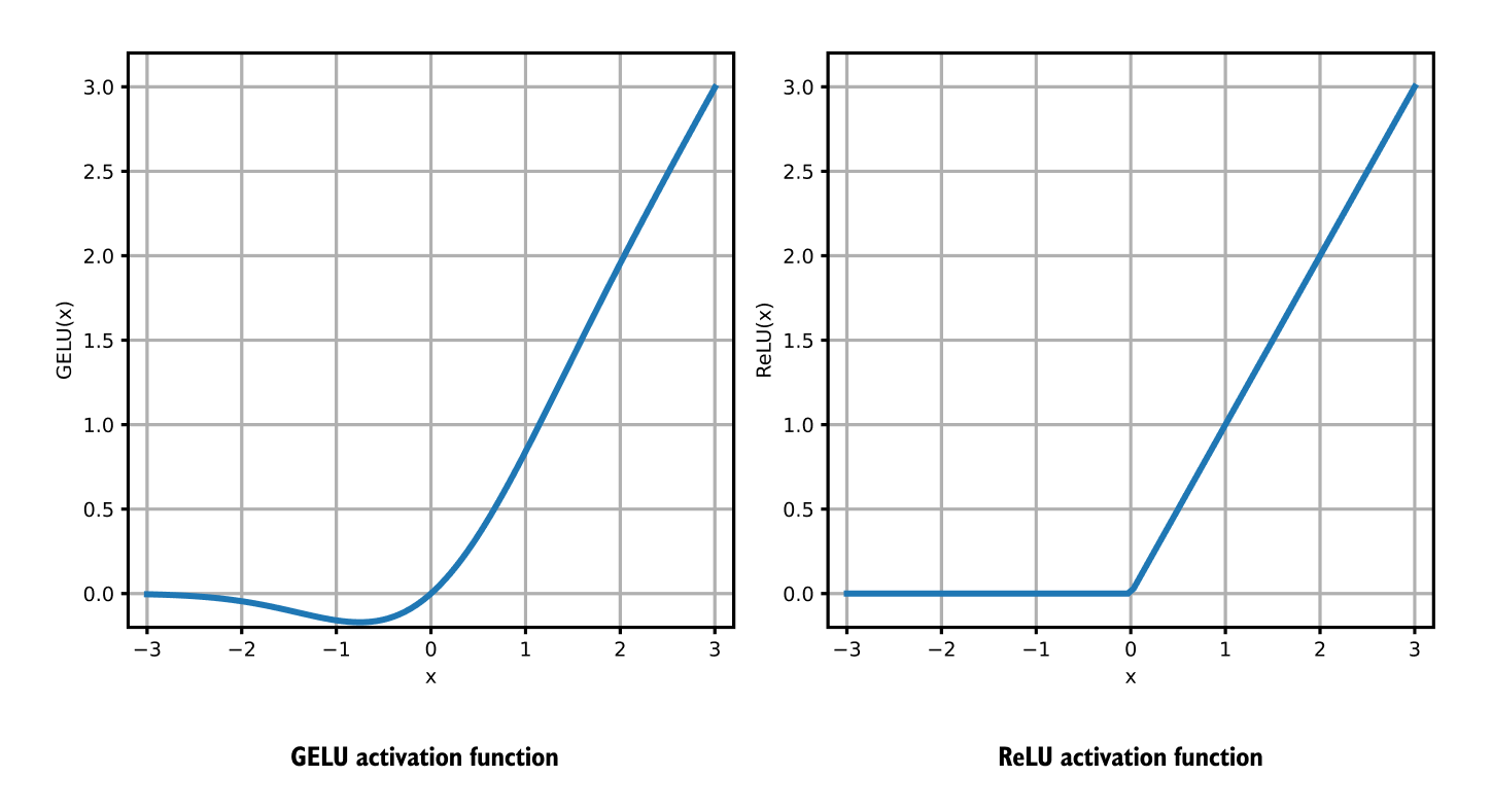
Figure 1.122: Comparison of ReLU and GELU activation functions. GELU is smooth everywhere, including at zero, and preserves small negative activations rather than collapsing them to exactly zero
After the expansion, the output is passed through a nonlinearity. Early transformer implementations used the ReLU activation function. ReLU simply returns x when x is positive and returns zero for negative x. Graphically, this is a straight line through the origin for positive inputs and a flat line at zero for negative inputs. ReLU is easy to implement and works well in many convolutional and fully connected networks, but it has two important drawbacks in this setting. First, every negative input is collapsed to exactly zero, so any information stored in the magnitude of negative activations is lost. If many units become negative, a large part of the network can effectively stop learning, a problem often described informally as dead neurons. Second, the ReLU curve has a sharp corner at zero and is not differentiable there. In practice we can still compute subgradients and train, but the function is not smooth.
Because of these issues, transformer language models have largely switched to the GELU activation. The GELU curve, shown next to ReLU in the figures, is a smooth S shaped function. For large positive inputs it behaves similarly to ReLU and returns values close to the identity. For large negative inputs it sends activations toward zero, so very negative units are still turned off. The important difference appears around zero. Instead of cutting everything below zero to exactly zero, GELU tapers smoothly and maps small negative inputs to small negative outputs. This has two consequences. First, the function is differentiable everywhere, including at zero, which makes optimization smoother. Second, the network does not discard all information carried by small negative activations. In the region near zero the model can still use their sign and magnitude to encode subtle distinctions. Together with layer normalization, which keeps activations in a moderate range and prevents very large negative or positive values, this leads to more stable training and slightly better performance in practice.
The output tensor of the feed forward network has exactly the same shape as its input, namely batch size, context length, embedding dimension. This design choice is deliberate. Because the main hidden dimension remains constant, we can add a residual connection around the feed forward sublayer and stack an arbitrary number of transformer blocks on top of each other without reshaping tensors. It becomes straightforward to plug in more blocks, remove blocks, or reuse the same block structure in very deep models, since every block expects and returns vectors of size 768 in this example.
It is also helpful to connect this back to the question of how many tokens the network sees at once. While the feed forward network operates on each token vector independently, each of those vectors already encodes information about the entire context window thanks to the preceding multi head attention. In our example with context length 3, the tensor has shape 2, 3, 768, and each of the three vectors for a given sequence summarizes that position in the context of the other positions. The feed forward network then applies a rich non linear transformation to each of these contextual vectors. When generating text autoregressively, the model still predicts one next token at a time, but this prediction is based on the full context representation, which has been refined by both attention and the feed forward expansion, activation and contraction.
In summary, the position wise feed forward network in a transformer block is a powerful per token multilayer perceptron. It expands the embedding dimension to a higher dimensional space, applies a smooth and information preserving GELU nonlinearity, and contracts the representation back to the original size. This structure provides most of the depth and nonlinearity in the model, while attention handles interaction across positions. Together they give transformers the capacity to learn complex patterns in sequences of tokens.
1.19 Shortcut connections
Layer normalization helps stabilize the scale of activations, but on its own it is not enough to reliably train very deep transformer stacks. In the previous section we saw that each block already contains a powerful feed forward network that expands the embedding dimension, applies a GELU nonlinearity, and then contracts it again. If we simply stacked many of these attention plus feed forward blocks, gradients flowing backward through all of those nonlinear layers would quickly become very small. To keep such deep transformers trainable, we rely on another key idea shortcut connections, also called residual connections.
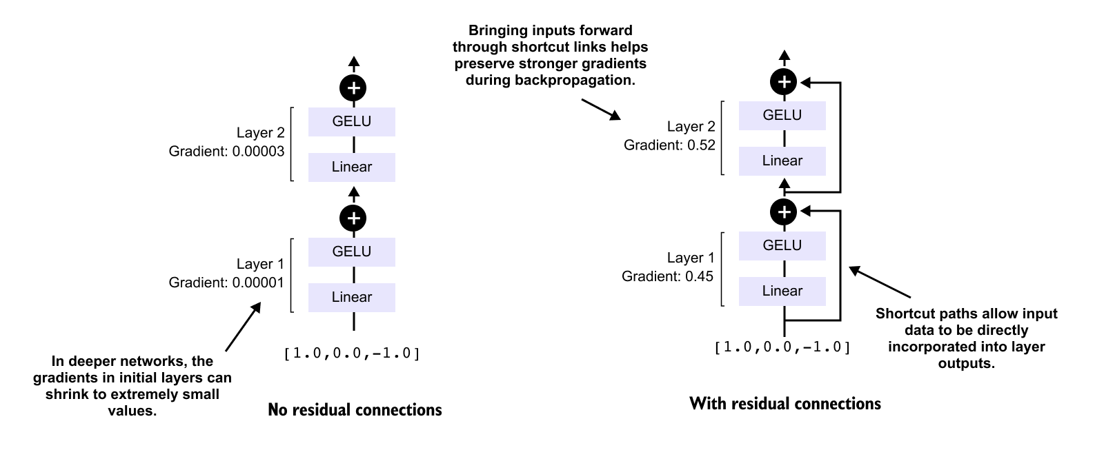
Figure 1.123: Effect of shortcut connections on gradients. Left: without shortcuts, gradients vanish (0.00003, 0.00001). Right: with shortcuts, gradients remain large (0.45, 0.52), enabling effective learning in earlier layers.
A shortcut connection simply adds the input of a block to its output, giving the signal an extra path through the model that bypasses one or more nonlinear layers. This extra path turns out to be very effective at keeping gradients from disappearing during backpropagation.
You can see the effect in the two layer illustration. On the left we have a small network that takes an input vector such as [1.0, 0.0, 0.0, minus 1.0], applies a linear layer and GELU activation twice, and then propagates gradients from the output back to the earlier layers. Without shortcut connections, the gradient at layer 2 might be around 0.00003 and at layer 1 around 0.00001. These tiny values are an example of the vanishing gradient problem the early layers barely receive any learning signal.
Now compare this to the version on the right, which adds residual connections around each linear plus GELU block. The same input is fed forward, but now the input of layer 1 is added to its output, and the output of layer 1 is added to the output of layer 2. With these shortcut paths in place, the gradients during backpropagation are much larger for the same network depth values like 0.45 for layer 1 and 0.52 for layer 2 in the illustration. Bringing the inputs forward through shortcut links preserves stronger gradients in the earlier layers, which makes learning much more effective.
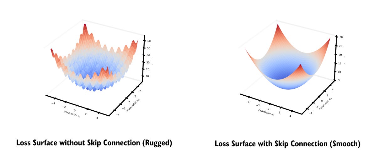
Figure 1.124: Loss landscape comparison: without skip connections the surface is jagged with many sharp peaks (left), while with skip connections the landscape becomes smooth with broad valleys (right).
There is also an optimization perspective that connects to the loss landscape illustration. If you visualize the loss of a deep network without shortcut connections as a function of its parameters, the surface often looks jagged, with many sharp peaks and narrow valleys. This makes gradient based optimization difficult and can trap training in poor local minima. When you add skip connections, the same network tends to exhibit a much smoother loss surface with broader valleys and fewer sharp spikes. A smoother landscape leads to more predictable gradients and makes it easier for simple optimizers like Adam to find good solutions.
Transformers exploit shortcut connections throughout the architecture. Within each transformer block, the input token representations are passed into a sublayer such as multi head attention or the feed forward network, and the sublayer output is added back to the original input. During backpropagation, gradients can then flow both through the sublayer and directly along the identity shortcut. This combination of residual paths and layer normalization is what allows transformers to stack many attention and feed forward blocks while still training reliably on large datasets.
1.20 Why Transformers Scale Better Than RNNs and CNNs
Transformers are fundamentally designed for scalability, both in terms of model size and training efficiency. Unlike recurrent neural networks, which process tokens sequentially and therefore suffer from limited parallelism, transformers operate on entire sequences at once. Self attention allows every token to directly interact with every other token in a single layer, removing the need to propagate information step by step through time. This parallel structure maps naturally to modern hardware such as GPUs and TPUs, enabling efficient utilization of large compute budgets. Compared to convolutional neural networks, which rely on fixed receptive fields and require deep stacks to capture long range dependencies, transformers model global context explicitly from the start. As models grow larger, this ability to combine global context with parallel computation leads to predictable improvements in performance, making transformers well suited for large scale training regimes.
Another key factor behind transformer scalability is architectural uniformity. The same transformer block can be stacked repeatedly with minimal modification, allowing depth and width to be increased systematically. Residual connections and normalization stabilize training even when hundreds of layers are used, while attention weights adapt dynamically to different inputs rather than being hard coded as in convolutions. This combination results in smooth scaling behavior where increasing parameters, data, and compute leads to consistent gains. In contrast, RNNs often struggle with vanishing gradients at scale, and CNNs require task specific architectural tuning. Transformers therefore provide a general purpose backbone that benefits directly from scale without extensive redesign.
1.21 Pretraining, Fine Tuning, and Transfer Learning in Transformers
Pretraining is the process that gives transformers their general purpose capabilities. In this stage, a model is trained on large amounts of unlabeled data using a self supervised objective such as next token prediction. The goal is not to solve a specific task, but to learn broad statistical structure in language or other modalities. During pretraining, the transformer learns representations that capture syntax, semantics, and long range dependencies. These representations are distributed across layers and attention heads, forming a reusable foundation that can support many downstream tasks. Because the objective is simple and data is abundant, pretraining scales effectively with model size and dataset size.
Fine tuning adapts a pretrained transformer to a specific task or domain. Instead of training from scratch, the pretrained weights are used as initialization, and training continues on a smaller labeled dataset. This process reshapes the learned representations toward task relevant patterns while preserving general knowledge acquired during pretraining. Transfer learning emerges naturally from this setup, since the same pretrained model can be reused across many tasks such as classification, generation, or question answering. In practice, this dramatically reduces data requirements and training time compared to building separate models for each task. It also enables rapid experimentation, since changes in objectives or datasets do not require redesigning the entire architecture.
1.22 Limitations and Challenges of Transformers
Despite their success, transformers are not without limitations. The most significant challenge lies in the quadratic cost of self attention with respect to sequence length. As input sequences grow longer, memory usage and computation increase rapidly, placing practical limits on context size. While various approximations and sparse attention mechanisms exist, they often introduce trade offs between efficiency and modeling fidelity. This makes long context modeling an active area of research rather than a solved problem.
Transformers also require substantial data and compute to reach their full potential. Large models trained on small or noisy datasets can overfit or learn spurious correlations, leading to unreliable behavior. In addition, pretrained transformers inherit biases present in their training data, which can surface during downstream use. From an engineering perspective, training and deploying large transformer models introduces challenges related to cost, latency, and energy consumption. These constraints mean that while transformers scale well in theory, practical deployments must balance model size with efficiency, reliability, and responsible use.
1.23 Hands On Coding a Miniature Transformer for Sequence Classification
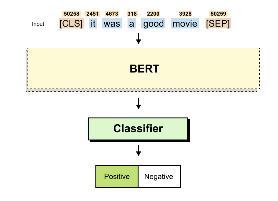
Figure 1.245: Sequence classification with BERT, where the input sentence is encoded, summarized by the classification token, and mapped by a classifier to a sentiment label.
The Notebook code is available here
https://github.com/VizuaraAI/Transformers-for-vision-BOOK
So far, we have discussed the transformer architecture and its core components at a conceptual level. To make these ideas concrete, we now move from theory to practice by implementing a small transformer model from scratch. The goal of this section is not to recreate a full scale BERT model, but to clearly understand how its fundamental design translates into working code.
In this hands on walkthrough, we build a miniature transformer for sequence classification using the IMDB movie review dataset. This dataset consists of textual reviews labeled with positive or negative sentiment, making it a practical and intuitive example for understanding how transformers process and classify entire sequences of text. Sequence classification highlights one of the key strengths of transformer encoders: their ability to capture bidirectional context across a complete input.
We will construct the model step by step, beginning with data loading and tokenization, then implementing embeddings, self attention, and transformer blocks, and finally adding a simple classification head. Each component is introduced explicitly so the flow of information through the model remains transparent. By the end of this section, you will have a working transformer classifier trained on the IMDB dataset and a clear understanding of how BERT style sequence classification models are built from scratch.
Listing 1.20: Installing the Required Dependencies
!pip install torch datasets tiktoken tqdm scikit-learnListing 1.21: Importing All Required Python Modules
import math
import os
import torch
import torch.nn as nn
import torch.nn.functional as F

from torch.utils.data import Dataset, DataLoader
from datasets import load_dataset
from tqdm import tqdm
import tiktoken

from sklearn.metrics import classification_report, confusion_matrix
Listing 1.22: Selecting the Compute Device
device = torch.device("cuda" if torch.cuda.is_available() else "cpu")
print(device)
Output
device(type='cuda')In Listing 1.20, we begin by installing the core dependencies required to implement a transformer based sequence classification model. PyTorch provides the foundational tensor operations and neural network abstractions that will be used to define embeddings, attention mechanisms, and training loops. The datasets library allows us to easily load the IMDB movie review dataset, while tiktoken supplies a modern subword tokenizer suitable for transformer models. The tqdm library is included to visualize training progress, and scikit learn provides standard evaluation utilities that will later help us interpret classification performance.
With the environment prepared, Listing 1.21 imports all required Python modules. In addition to standard libraries such as math and os, we import PyTorch’s neural network components, including layers, activation functions, and data loading utilities. The Dataset and DataLoader classes define how text samples are structured and batched during training. The load_dataset function simplifies dataset retrieval, and tqdm enables progress tracking during training iterations. Finally, evaluation tools such as classification reports and confusion matrices are imported to support quantitative analysis of model predictions after training.
Finally, in Listing 1.22, we select the compute device on which the model will run. The code checks whether a CUDA enabled GPU is available and assigns it as the execution device when possible, otherwise defaulting to the CPU. This conditional setup allows the same implementation to scale from local experimentation to accelerated training environments without modification. With the dependencies installed, modules imported, and the compute device configured, we have established a solid foundation for building and training a transformer model from scratch in the sections that follow.
Before building the transformer model, we first need a dataset that clearly illustrates the sequence classification task. In this section, we use the IMDB movie review dataset, a widely used benchmark for sentiment analysis. The dataset contains 50,000 movie reviews split evenly into training and test sets. Each review is labeled with one of two classes: positive sentiment or negative sentiment. The text samples vary in length and style, ranging from short opinions to long, detailed critiques, which makes the dataset well suited for evaluating a model’s ability to understand full sequences of natural language. A typical sample consists of a review such as
“The movie was slow, but the performances were outstanding,” paired with a binary label indicating its sentiment.
Listing 1.23: Loading the IMDb Dataset
dataset = load_dataset("imdb")

train_texts = dataset["train"]["text"]
train_labels = dataset["train"]["label"]

test_texts = dataset["test"]["text"]
test_labels = dataset["test"]["label"]

len(train_texts), len(test_texts)
Output
(25000, 25000)In Listing 1.23, we load the IMDB dataset using the datasets library, which automatically downloads and prepares the data in a standardized format. The dataset is split into training and test partitions, each containing 25,000 samples. From each split, we extract the raw review texts and their corresponding sentiment labels. The labels are encoded as integers, where 0 represents negative sentiment and 1 represents positive sentiment. At this stage, the data remains in raw text form, which allows us to apply custom tokenization and preprocessing steps in later sections.
Listing 1.24: Initializing a Byte Pair Encoding Tokenizer
tokenizer = tiktoken.get_encoding("gpt2")
base_vocab_size = tokenizer.n_vocab
base_vocab_size
Output
50257In Listing 1.24, we initialize a Byte Pair Encoding tokenizer using the GPT 2 vocabulary. As discussed earlier in the tokenization section. The GPT 2 tokenizer comes with a fixed base vocabulary size of 50,257 tokens, which includes common words, subwords, punctuation, and special byte level encodings. We reuse this tokenizer to avoid designing a vocabulary from scratch and to ensure efficient coverage of the diverse language found in movie reviews. Here, we record the base vocabulary size because we will extend it in the next step.
Preparing Text Inputs and Batches for Transformers
Before introducing special tokens and moving into the BERT specific input construction, we first need to understand how raw text is transformed into batches that a transformer can process. Transformers do not operate directly on free form text. Instead, text must pass through a sequence of structured transformations that determine what the model sees as input and what it is trained to predict.
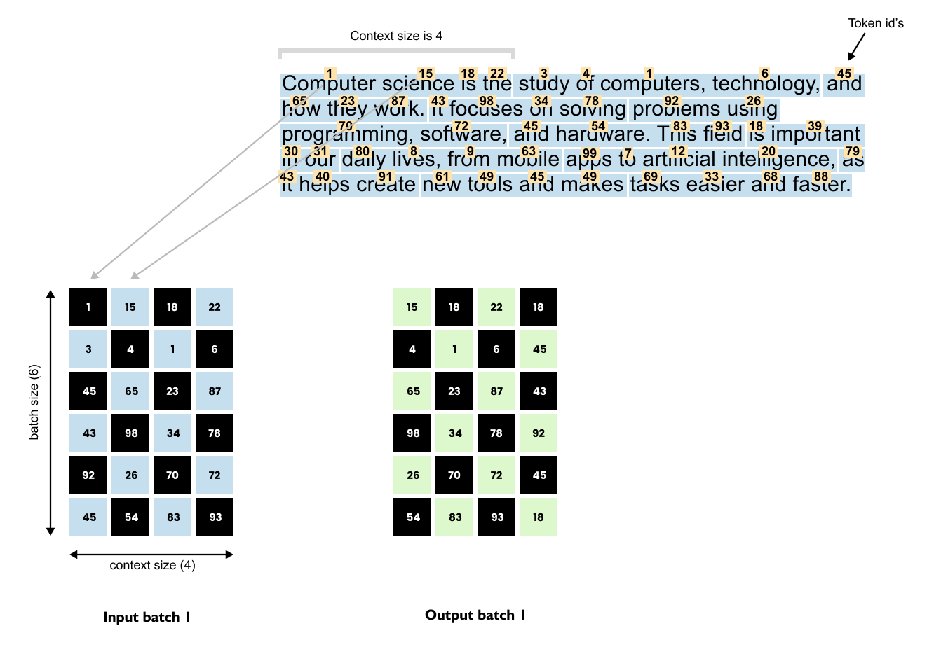
Figure 1.246: Preparing text for a transformer: raw text is tokenized, split into context windows, and arranged into input–output batch pairs where each target is the next token.
We begin with a continuous piece of text, which is first broken into tokens. In the example shown in Figure, each word in the paragraph is mapped to a corresponding token id. At this stage, the text is still treated as one long sequence. Because transformers have a fixed context size, the model cannot process the entire sequence at once. Instead, a context window is chosen, which defines how many consecutive tokens the model can attend to in a single forward pass.
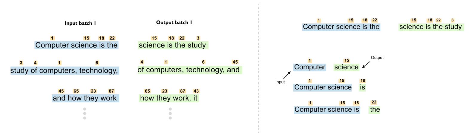
Figure 1.247: Sliding window mechanism: the token sequence is sliced into overlapping segments, each becoming one training example where the output is the input shifted by one position
Using this fixed context window, the token sequence is sliced into overlapping segments. Each segment becomes one training example. As illustrated in Figure, the input batch contains sequences of tokens within the context window, while the output batch contains the same sequences shifted by one position. This shift is the learning signal. The model is trained to predict the next token at every position, which is why the input and output batches appear nearly identical except for alignment.
If you will see the second figure, each row in the input batch corresponds to a short phrase extracted from the original sentence, and each row in the output batch represents the immediate continuation of that phrase. This sliding window mechanism allows a single sentence to generate many training examples. When these examples are stacked together, they form a batch that can be processed efficiently in parallel by the transformer.
The figure highlights an important property of next token prediction. The model does not predict only the final word of a sentence. Instead, it learns to predict the next token at every position, given the context seen so far. This is why context grows incrementally and why causal masking is required in autoregressive models. At each step, the model is only allowed to attend to previous tokens within the context window.
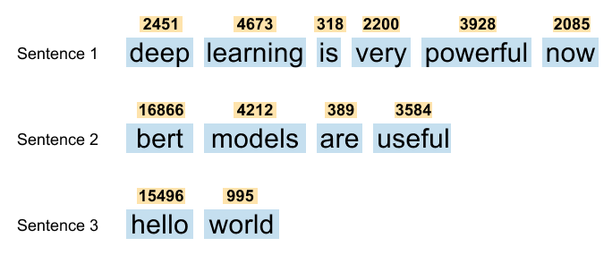
Figure 1.248: For BERT-style classification, multiple independent sentences are tokenized separately, producing sequences of different lengths.
The next transition shown in this figure moves away from next token prediction and toward sequence level processing. Here, we start with multiple independent sentences rather than one long document. Each sentence is tokenized separately, producing sequences of different lengths. At this stage, these sequences cannot yet be processed together because transformers require all inputs in a batch to share the same length.
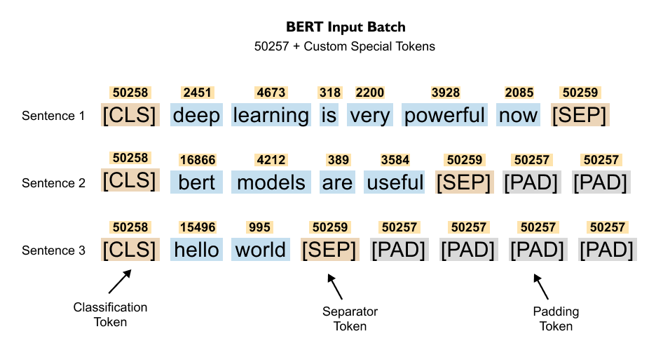
Figure 1.249: BERT input formatting: a classification token is added at the beginning, a separator token at the end, and padding tokens fill shorter sequences to a uniform length.
See in this figure how BERT resolves this issue through structured input formatting. Each sentence is augmented with a classification token at the beginning and a separator token at the end. Shorter sequences are padded so that all examples reach the same length. Padding tokens do not represent real text and are later ignored by attention masks, but they are essential for forming a rectangular batch tensor.
Listing 1.25: Extending the Tokenizer with BERT Special Tokens
PAD_ID = base_vocab_size
CLS_ID = base_vocab_size + 1
SEP_ID = base_vocab_size + 2

VOCAB_SIZE = base_vocab_size + 3
VOCAB_SIZE
Output
50260The classification token introduced here plays a special role. During self attention, it attends to all other tokens in the sequence, allowing it to accumulate information from the entire sentence. By the final transformer layer, its hidden state acts as a compact summary of the sequence. This is the representation used for sequence classification tasks such as sentiment analysis.
This progression, from sliding context windows for next token prediction to padded, sentence level batches for BERT style processing, illustrates a critical shift in how transformers consume text. Autoregressive models learn by predicting future tokens, while BERT learns by encoding entire sequences at once. With this conceptual foundation established, we are now ready to formally introduce special tokens in the code and explain their precise role in the BERT implementation.
By appending these tokens after the original GPT 2 vocabulary, we preserve all existing token mappings while expanding the vocabulary size to 50,260. This setup allows the transformer model to handle variable length inputs and perform sequence level classification in a manner consistent with BERT style architectures.
Listing 1.26: Encoding Text into Fixed-Length BERT Input Sequences
MAX_LEN = 256

def encode(text):
    token_ids = tokenizer.encode(text)
    token_ids = token_ids[:MAX_LEN - 2]

    token_ids = [CLS_ID] + token_ids + [SEP_ID]

    if len(token_ids) < MAX_LEN:
        token_ids += [PAD_ID] * (MAX_LEN - len(token_ids))

    return token_ids
This function converts raw text into a fixed length input sequence that the BERT model can process. The text is first tokenized into subword token ids using the tokenizer, and the sequence is truncated to leave space for the special tokens. A classification token is then added to the beginning of the sequence and a separator token to the end, establishing clear boundaries for the model. If the resulting sequence is shorter than the maximum length, padding tokens are appended until the desired length is reached. The output is a uniform length token sequence, which ensures that all inputs can be stacked into batches and processed efficiently by the transformer.
Note on Sequence Length: We limit the sequence length to 256 tokens to maintain training efficiency, as the self-attention mechanism’s computational cost grows quadratically
While this speeds up processing, it uses “head-only” truncation which risks discarding important sentiment cues often found at the end of reviews; a “head+tail” strategy (keeping the first and last chunks) is often a more effective alternative for longer documents.
However, this is just a demonstration. If you want to increase accuracy, you can keep the entire text, but be aware that this will significantly increase training hours and computational costs.
Listing 1.27: Creating Attention Masks for Padding Tokens
def create_attention_mask(input_ids):
    return (input_ids != PAD_ID).long()
This function constructs an attention mask that distinguishes real tokens from padding tokens. Each position containing a padding token is marked with zero, while all other positions are marked with one. During self attention, this mask ensures that padded positions are ignored so they do not influence the model’s representations. Attention masks are essential when batching variable length sequences, as they allow the transformer to operate on padded inputs without learning from artificial padding.
Listing 1.28: Defining the IMDb Dataset Class
class IMDBDataset(Dataset):
    def __init__(self, texts, labels):
        self.texts = texts
        self.labels = labels

    def __len__(self):
        return len(self.texts)

    def __getitem__(self, idx):
        ids = torch.tensor(encode(self.texts[idx]))
        mask = create_attention_mask(ids)
        label = torch.tensor(self.labels[idx])

        return ids, mask, label
This dataset class wraps the raw text and labels into a format compatible with PyTorch training loops. For each example, the text is encoded into a fixed length token sequence, an attention mask is generated, and the corresponding label is returned. By centralizing encoding and masking inside the dataset, the data pipeline remains clean and consistent, ensuring that every batch fed into the model follows the same preprocessing logic.
Listing 1.29: Creating DataLoaders for Training and Evaluation
train_ds = IMDBDataset(train_texts, train_labels)
test_ds = IMDBDataset(test_texts, test_labels)

train_loader = DataLoader(train_ds, batch_size=16, shuffle=True)
test_loader = DataLoader(test_ds, batch_size=16)
Here, the dataset objects are passed into DataLoader instances, which handle batching and shuffling automatically. The training data is shuffled to prevent the model from learning order based artifacts, while the evaluation data is kept deterministic. DataLoaders enable efficient iteration over the dataset and ensure that inputs, masks, and labels are delivered to the model in properly structured batches.
Listing 1.30: Implementing the BERT Embedding Layer
class BERTEmbedding(nn.Module):
    def __init__(self, vocab_size, embed_dim, max_len, dropout=0.1):
        super().__init__()
        self.token = nn.Embedding(vocab_size, embed_dim, padding_idx=PAD_ID)
        self.position = nn.Embedding(max_len, embed_dim)
        self.segment = nn.Embedding(2, embed_dim)
        self.norm = nn.LayerNorm(embed_dim)
        self.dropout = nn.Dropout(dropout)

    def forward(self, x):
        B, T = x.size()
        pos = torch.arange(T).unsqueeze(0).to(x.device)
        seg = torch.zeros_like(x)

        embeddings = (
            self.token(x) +
            self.position(pos) +
            self.segment(seg)
        )

        embeddings = self.norm(embeddings)
        embeddings = self.dropout(embeddings)
        return embeddings
This module implements the embedding layer used in BERT style models. Token embeddings encode word identity, positional embeddings capture word order, and segment embeddings provide sentence level context, even though a single segment is used here. These embeddings are summed to form the input representation for the transformer encoder. Layer normalization and dropout are applied to stabilize training and improve generalization. This embedding layer serves as the entry point where raw token ids are transformed into dense vectors suitable for self attention.
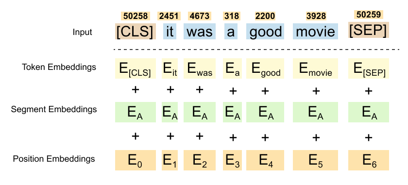
Figure 1.250: BERT input representation for single-sentence IMDb classification, showing token embeddings (CLS + tokens + SEP), uniform segment A embeddings across all tokens (used consistently despite single sentence to maintain pre-training format for sentence A/B distinction), and positional embeddings summed together.
Listing 1.31: Implementing Multi-Head Self-Attention
class MultiHeadSelfAttention(nn.Module):
    def __init__(self, dim, heads, dropout=0.1):
        super().__init__()
        assert dim % heads == 0

        self.heads = heads
        self.d = dim // heads

        self.qkv = nn.Linear(dim, dim * 3)
        self.out = nn.Linear(dim, dim)

        self.attn_dropout = nn.Dropout(dropout)
        self.out_dropout = nn.Dropout(dropout)

    def forward(self, x, mask):
        B, T, C = x.shape

        q, k, v = self.qkv(x).chunk(3, dim=-1)

        q = q.view(B, T, self.heads, self.d).transpose(1, 2)
        k = k.view(B, T, self.heads, self.d).transpose(1, 2)
        v = v.view(B, T, self.heads, self.d).transpose(1, 2)

        scores = (q @ k.transpose(-2, -1)) / math.sqrt(self.d)

        mask = mask.unsqueeze(1).unsqueeze(2)
        scores = scores.masked_fill(mask == 0, -1e9)

        attn = F.softmax(scores, dim=-1)
        attn = self.attn_dropout(attn)

        out = attn @ v
        out = out.transpose(1, 2).reshape(B, T, C)

        out = self.out(out)
        out = self.out_dropout(out)
        return out
This module implements the core self attention mechanism used inside BERT. The input embeddings are first projected into queries, keys, and values using a single linear layer and then split across multiple attention heads. Each head operates on a smaller subspace of the embedding dimension, allowing the model to attend to different relationships in parallel. Scaled dot product attention is applied within each head, and the attention mask is used to prevent padded tokens from contributing to the computation. The outputs of all heads are then concatenated, projected back to the original embedding dimension, and passed through dropout for regularization.
The key architectural difference between this BERT style attention and the attention used in GPT lies in masking. In BERT, self attention is fully bidirectional, meaning every token is allowed to attend to every other token in the sequence. The only masking applied here is to ignore padding tokens. In contrast, GPT uses causal masking to prevent tokens from attending to future positions, enforcing an autoregressive left to right structure. Aside from this masking behavior, the mathematical formulation of multi head self attention remains the same across both architectures.
Listing 1.32: Implementing the Feed-Forward Network
class FeedForward(nn.Module):
    def __init__(self, dim, hidden, dropout=0.1):
        super().__init__()
        self.net = nn.Sequential(
            nn.Linear(dim, hidden),
            nn.GELU(),
            nn.Dropout(dropout),
            nn.Linear(hidden, dim),
            nn.Dropout(dropout)
        )

    def forward(self, x):
        return self.net(x)
This module defines the position wise feed forward network used inside each transformer encoder layer. After self attention mixes information across tokens, the feed forward network independently transforms each token representation using the same set of parameters. It consists of two linear projections with a GELU activation in between, which introduces nonlinearity and allows the model to learn more expressive feature transformations. Dropout is applied after each linear layer to reduce overfitting and improve generalization. Although simple in structure, this feed forward network plays a critical role by refining token representations at every layer and complementing the relational modeling performed by self attention.
Listing 1.33: Defining a Transformer Encoder Block
class TransformerBlock(nn.Module):
    def __init__(self, dim, heads, ff_dim, dropout=0.1):
        super().__init__()
        self.attn = MultiHeadSelfAttention(dim, heads, dropout)
        self.ff = FeedForward(dim, ff_dim, dropout)
        self.norm1 = nn.LayerNorm(dim)
        self.norm2 = nn.LayerNorm(dim)

    def forward(self, x, mask):
        x = x + self.attn(self.norm1(x), mask)
        x = x + self.ff(self.norm2(x))
        return x
This module brings together the two fundamental components of the transformer encoder into a single reusable block. Each block first applies multi head self attention to allow tokens to exchange information across the sequence, and then applies a position wise feed forward network to refine each token representation independently. Layer normalization is applied before each sublayer to stabilize training, while residual connections add the sublayer outputs back to the original input. This design preserves gradient flow in deep networks and enables stacking many encoder blocks without degradation. By repeatedly applying this block, the model progressively builds richer and more contextual representations of the input sequence, which is the core mechanism behind BERT style encoders.
Listing 1.34: Constructing the BERT Encoder Stack
class BERTEncoder(nn.Module):
    def __init__(self, vocab_size, dim, max_len, layers, heads, ff_dim):
        super().__init__()
        self.embed = BERTEmbedding(vocab_size, dim, max_len)
        self.layers = nn.ModuleList([
            TransformerBlock(dim, heads, ff_dim)
            for _ in range(layers)
        ])

    def forward(self, x, mask):
        x = self.embed(x)
        for layer in self.layers:
            x = layer(x, mask)
        return x
After defining the embedding layer and the transformer encoder block, we can now assemble the complete BERT encoder. This step connects all the components introduced so far into a single coherent module. The encoder begins by converting input token ids into dense vector representations using the BERT embedding layer, which injects token identity, positional information, and segment context. These embeddings serve as the initial representation of the input sequence.
Once the embeddings are formed, they are passed through a stack of transformer encoder blocks. Each block applies multi head self attention to mix information across tokens, followed by a feed forward network to refine each token representation. By stacking multiple such blocks, the model repeatedly contextualizes the sequence, allowing higher layers to build on patterns discovered in earlier ones. The output of the encoder is a sequence of deeply contextualized token embeddings, where each token representation reflects information from the entire input. This encoder stack forms the core of the BERT architecture and provides the representations that will later be used for sequence level classification.
Listing 1.35: Adding a Sequence Classification Head
class BERTForClassification(nn.Module):
    def __init__(self, vocab_size, dim, max_len, layers, heads, ff_dim):
        super().__init__()
        self.bert = BERTEncoder(
            vocab_size, dim, max_len, layers, heads, ff_dim
        )
        self.classifier = nn.Sequential(nn.Dropout(0.1),nn.Linear(dim, 2))

    def forward(self, x, mask):
        out = self.bert(x, mask)
        cls = out[:, 0]
        return self.classifier(cls)
With the BERT encoder stack in place, the final step is to adapt it for a concrete downstream task. In this module, we attach a lightweight sequence classification head on top of the encoder. The encoder itself remains unchanged and continues to produce contextualized embeddings for every token in the input sequence. What is new here is how we convert those token level representations into a single prediction.
During the forward pass, the output of the BERT encoder is a tensor containing one embedding per token. We explicitly select the representation of the first token in the sequence, which corresponds to the classification token introduced earlier. As discussed previously, this token has attended to all other tokens through self attention and therefore acts as a compact summary of the entire sequence. The classification head applies dropout for regularization and then uses a linear layer to map this summary representation to class logits. This design cleanly separates general language encoding from task specific prediction, allowing the same encoder to be reused for different classification tasks with minimal modification.
Listing 1.36: Initializing the Model
model = BERTForClassification(
    vocab_size=VOCAB_SIZE,
    dim=256,
    max_len=MAX_LEN,
    layers=4,
    heads=6,
    ff_dim=1024
).to(device)

print(model)
Output
BERTForClassification(
  (bert): BERTEncoder(
    (embed): BERTEmbedding(
      (token): Embedding(50260, 256, padding_idx=50257)
      (position): Embedding(256, 256)
      (segment): Embedding(2, 256)
      (norm): LayerNorm((256,), eps=1e-05, elementwise_affine=True)
      (dropout): Dropout(p=0.1, inplace=False)
    )
    (layers): ModuleList(
      (0-5): 6 x TransformerBlock(
        (attn): MultiHeadSelfAttention(
          (qkv): Linear(in_features=256, out_features=768, bias=True)
          (out): Linear(in_features=256, out_features=256, bias=True)
          (attn_dropout): Dropout(p=0.1, inplace=False)
          (out_dropout): Dropout(p=0.1, inplace=False)
        )
        (ff): FeedForward(
          (net): Sequential(
            (0): Linear(in_features=256, out_features=1024, bias=True)
            (1): GELU(approximate='none')
            (2): Dropout(p=0.1, inplace=False)
            (3): Linear(in_features=1024, out_features=256, bias=True)
            (4): Dropout(p=0.1, inplace=False)
          )
        )
        (norm1): LayerNorm((256,), eps=1e-05, elementwise_affine=True)
        (norm2): LayerNorm((256,), eps=1e-05, elementwise_affine=True)
      )
    )
  )
  (classifier): Sequential(
    (0): Dropout(p=0.1, inplace=False)
    (1): Linear(in_features=256, out_features=2, bias=True)
  )
)
Finally, we are ready to define the complete model by bringing together all the components built so far. At this stage, the embedding layer, transformer encoder stack, and sequence classification head are no longer independent pieces but parts of a single, end to end architecture.
The model is initialized with an embedding dimension of 256, which determines the size of the vector representation used throughout the network. Four transformer encoder layers are stacked to progressively refine contextual information, while six attention heads in each layer allow the model to capture multiple relationships in parallel. Inside each layer, the feed forward network expands the representation to 1024 dimensions before projecting it back, preserving the standard transformer design pattern. The vocabulary size includes both the base tokenizer and the added BERT specific special tokens, and the maximum sequence length defines the longest input the model can process.
Once instantiated, the model is moved to the selected compute device, completing the setup phase. With the architecture now fully defined, the BERT model is ready to be trained on the IMDB dataset, marking the transition from model construction to optimization.
Listing 1.37: Defining the Loss Function and Optimizer
With the model architecture fully defined and instantiated, we now set up the two components needed for training: the loss function and the optimizer.
For the loss function, we use `CrossEntropyLoss`, which is the standard choice for classification tasks. Cross-entropy loss measures the difference between the model’s predicted probability distribution over the two classes (positive and negative sentiment) and the true label. Internally, PyTorch’s `CrossEntropyLoss` applies the softmax function to the raw logits produced by the model and then computes the negative log likelihood, so we do not need to apply softmax ourselves before passing the logits to the loss function.
criterion = nn.CrossEntropyLoss()
optimizer = torch.optim.AdamW(model.parameters(), lr=3e-4)
AdamW
Adam optimizers are a popular choice for training deep neural networks. However, in our training loop, we opt for the AdamW optimizer. AdamW is a variant of Adam that improves the weight decay approach, which aims to minimize model complexity and prevent overfitting by penalizing larger weights. This adjustment allows AdamW to achieve more effective regularization and better generalization; thus, AdamW is frequently used in the training of transformer models.
Listing 1.38: Training the Model
EPOCHS = 100

for epoch in range(EPOCHS):
    model.train()
    total_loss = 0

    for ids, mask, labels in tqdm(train_loader):
        ids, mask, labels = ids.to(device), mask.to(device), labels.to(device)

        optimizer.zero_grad()
        logits = model(ids, mask)
        loss = criterion(logits, labels)
        loss.backward()
        optimizer.step()

        total_loss += loss.item()

    print(f"Epoch {epoch+1} | Train Loss: {total_loss:.2f}")
Output (abbreviated)
Epoch 1 | Train Loss: 1078.51
Epoch 2 | Train Loss: 1040.23
Epoch 3 | Train Loss: 1009.87
...
Epoch 50 | Train Loss: 512.34
...
Epoch 98 | Train Loss: 289.45
Epoch 99 | Train Loss: 287.12
Epoch 100 | Train Loss: 285.67
It is now time to implement the training loop. The training process follows the standard PyTorch pattern: for each epoch, we iterate over all batches in the training DataLoader, compute the forward pass to obtain logits, calculate the loss, perform backpropagation to compute gradients, and update the model parameters using the optimizer.
At the beginning of each epoch, we set the model to training mode using model.train(). This ensures that layers such as Dropout and LayerNorm behave correctly during training, dropout randomly zeroes elements to prevent overfitting, and layer normalization uses batch-level statistics. At the start of each batch, we call optimizer.zero_grad() to reset the gradients accumulated from the previous iteration, since PyTorch accumulates gradients by default. The forward pass produces logits from the model, the loss is computed against the true labels, and loss.backward() calculates the gradients through backpropagation. Finally, optimizer.step() updates all model parameters using the computed gradients.
We train for a relatively large number of epochs to allow the small model to converge. The cumulative loss over all batches is printed at the end of each epoch to monitor training progress. A decreasing loss across epochs indicates that the model is successfully learning to distinguish positive from negative reviews.
As we can see from the output, the training loss decreases steadily across epochs, indicating that the model is learning meaningful representations from the training data. The loss starts high in the first epoch because the model’s weights are randomly initialized and the predictions are essentially random guesses. Over the course of training, the model adjusts its parameters to produce increasingly accurate sentiment predictions.
Note on Training Duration:
Training for 100 epochs on 25,000 samples with a batch size of 16 results in approximately 156,250 parameter updates per epoch. On a modern GPU, this takes several hours. If computational resources are limited, reducing the number of epochs to 10–20 will still produce a model that performs noticeably above chance, though with lower accuracy.
Listing 1.39: Evaluating the Model on the Test Set
def evaluate(model, loader):
    model.eval()
    correct, total = 0, 0

    with torch.no_grad():
        for ids, mask, labels in loader:
            ids, mask, labels = ids.to(device), mask.to(device), labels.to(device)
            preds = model(ids, mask).argmax(dim=1)

            correct += (preds == labels).sum().item()
            total += labels.size(0)

    return correct / total
accuracy = evaluate(model, test_loader)
print("Test Accuracy:", accuracy)Output
Test Accuracy: 0.8074After training, we evaluate the model on the held-out test set to measure its generalization performance, that is, how well it classifies reviews it has never seen during training. This is a critical step, because a model that performs well on training data but poorly on unseen data has overfit to the training set and has not learned generalizable patterns.
During evaluation, we set the model to evaluation mode using model.eval(), which disables dropout and ensures that layer normalization uses its learned running statistics rather than batch-level statistics. We also wrap the evaluation loop inside torch.no_grad(), which disables gradient computation. Since we are not updating the model’s parameters during evaluation, disabling gradients reduces memory usage and speeds up computation.
For each batch, the model produces logits, and we take the argmax along the class dimension to obtain the predicted label (0 for negative, 1 for positive). We then compare these predictions to the ground truth labels and accumulate the number of correct predictions to compute the overall accuracy.
The model achieves approximately 80.7% accuracy on the test set. Considering that this is a BERT model trained entirely from scratch with a reduced architecture (256-dimensional embeddings, 4 layers, and 6 attention heads) on truncated input sequences of just 256 tokens, this is a reasonable result. For reference, the original BERT-Base model (768-dimensional embeddings, 12 layers, 12 heads) pretrained on massive corpora and then fine-tuned on IMDb typically achieves around 93–95% accuracy. The gap in performance is expected, given the significant differences in model size, pretraining data, and input sequence length.
Listing 1.40: Generating a Detailed Classification Report
While overall accuracy gives a useful single-number summary, it can sometimes be misleading, especially on imbalanced datasets. To get a more detailed picture of the model’s performance, we generate a full classification report using scikit-learn’s classification_report function. This report includes precision, recall, and F1-score for each class.
Precision measures what fraction of the samples the model predicted as a given class actually belong to that class. Recall measures what fraction of the samples that truly belong to a given class were correctly identified by the model. The F1-score is the harmonic mean of precision and recall, providing a single metric that balances both concerns. These per-class metrics are especially informative when the classes have different distributions or when the cost of false positives and false negatives differs.
To generate this report, we first collect all predictions and ground truth labels from the test set by running the model in evaluation mode with gradients disabled.
all_preds, all_labels = [], []

model.eval()
with torch.no_grad():
    for ids, mask, labels in test_loader:
        preds = model(ids.to(device), mask.to(device)).argmax(dim=1).cpu()
        all_preds.extend(preds.numpy())
        all_labels.extend(labels.numpy())

print(classification_report(all_labels, all_preds, target_names=["Negative", "Positive"]))
Output
              precision    recall  f1-score   support

    Negative       0.81      0.80      0.81     12500
    Positive       0.81      0.81      0.81     12500

    accuracy                           0.81     25000
   macro avg       0.81      0.81      0.81     25000
weighted avg       0.81      0.81      0.81     25000
The classification report confirms that the model performs consistently across both classes. The precision, recall, and F1-scores are all approximately 0.81 for both the negative and positive classes, with balanced support of 12,500 samples each. This symmetry indicates that the model does not exhibit a bias toward predicting one class over the other, which is a desirable property in a balanced binary classification task.
Listing 1.41: Saving the Trained Model
After training and evaluation, it is important to save the model so that it can be loaded later for inference or further fine-tuning without having to retrain from scratch. In PyTorch, the standard approach is to save the model’s state_dict, which is a Python dictionary that maps each layer name to its corresponding parameter tensor. Saving the state_dict rather than the entire model object is the recommended practice because it is more portable and less prone to issues when the code structure changes between sessions.
In addition to the model weights, we also save the tokenizer metadata, specifically the special token IDs and maximum sequence length, so that all the information needed for inference is available in one place. This ensures reproducibility: anyone who loads the model later will have the exact configuration required to tokenize new inputs in the same way they were processed during training.
SAVE_DIR = "bert_from_scratch_imdb"
os.makedirs(SAVE_DIR, exist_ok=True)

torch.save(model.state_dict(), f"{SAVE_DIR}/model.pt")

torch.save({
    "pad_id": PAD_ID,
    "cls_id": CLS_ID,
    "sep_id": SEP_ID,
    "max_len": MAX_LEN
}, f"{SAVE_DIR}/tokenizer_info.pt")

print("Model saved successfully!")
Output
Model saved successfully!Listing 1.42: Loading the Saved Model for Inference
Before running inference on new text, we load the saved model weights back into the model architecture. The torch.load function reads the saved state_dict from disk, and model.load_state_dict() applies these weights to the model. The map_location argument ensures that the weights are loaded onto the correct device, which is particularly useful when a model trained on a GPU is later loaded on a CPU-only machine.
After loading, we set the model to evaluation mode with model.eval(). This is essential because, without it, dropout layers would still randomly zero out activations, leading to inconsistent and degraded predictions at inference time.
model.load_state_dict(torch.load(f"{SAVE_DIR}/model.pt", map_location=device))
model.eval()
print("Model loaded successfully!")
Output
Model loaded successfully!Listing 1.43: Running Inference on New Text
With the trained model loaded, we can now use it to classify the sentiment of arbitrary text inputs. The inference pipeline mirrors the preprocessing steps used during training: the raw text is tokenized using byte pair encoding, augmented with classification and separator tokens, padded to the fixed sequence length, and converted into a tensor. An attention mask is created to indicate which positions contain real tokens versus padding. The model then produces logits for the two classes, and we take the argmax to obtain the predicted label.
We test the model on multiple example sentences, to verify that it has learned meaningful sentiment representations.
Some of the examples are
text = "Bromwell High is a brilliantly conceived, executed and acted, but sadly overlooked sitcom. The writing is razor sharp, the characters are well drawn and the jokes are genuinely funny. The animation is also excellent, with a style that suits the material perfectly. It's a shame that it didn't get a proper chance in the UK, as it deserves to be up there with the likes of The Simpsons and South Park. Highly recommended for anyone who likes clever, witty humour."

ids = torch.tensor([encode(text)]).to(device)
mask = (ids != PAD_ID).long()

with torch.no_grad():
    pred = model(ids, mask).argmax(dim=1).item()

print("Prediction:", "Positive" if pred == 1 else "Negative")
Output
Prediction: Positivetext = "In fact I must confess, so bad was it I fast forwarded through most of the garbage... As for the title characters, they barely even have a footnote in the film."
ids = torch.tensor([encode(text)]).to(device)
mask = (ids != PAD_ID).long()
with torch.no_grad():
pred = model(ids, mask).argmax(dim=1).item()
print("Prediction:", "Positive" if pred == 1 else "Negative")Output
Prediction: NegativeAs the outputs show, the model correctly classifies all two test inputs. The strongly positive reviews are predicted as positive, and the clearly negative reviews are predicted as negative. While these examples contain relatively unambiguous sentiment cues, they demonstrate that the model has learned to associate specific linguistic patterns, such as words like “brilliantly,” “excellent,” and “highly recommended” with positive sentiment, and phrases like “waste of time,” “cringe-worthy,” and “garbage” with negative sentiment.
It is worth noting that a small model trained from scratch on truncated sequences will not handle every edge case perfectly. Reviews with mixed sentiment, heavy sarcasm, or critical information located beyond the 256-token truncation point may be misclassified. Nonetheless, the model’s ability to correctly classify straightforward examples confirms that the BERT architecture, even at a reduced scale, can learn meaningful bidirectional representations for sentiment analysis when trained on a sufficiently large labeled dataset.
Resources
Dr Raj has made a very detailed playlist to built an LLM from Scratch, You could refer that as well
Also You can refer the book by Sebastian Raschka
Build a Large Language Model (From Scratch)
1.24 Summary
Large Language Models predict the next word in a sequence and use this simple objective to develop sophisticated language understanding. Model size is critical: emergent abilities such as arithmetic reasoning appear only when models cross certain parameter thresholds.
The transformer architecture replaces recurrent and convolutional approaches with self-attention, enabling parallel processing and global context from the first layer. Its core components are tokenization, embeddings, multi-head attention, feed-forward networks, layer normalization, and residual connections.
Byte Pair Encoding builds a subword vocabulary through iterative merging of 90, The Transformer Architecture the most frequent character pairs, balancing vocabulary size with the ability to represent any text.
Self-attention transforms static input embeddings into dynamic context vectors by projecting them into queries, keys, and values. Attention scores are computed via scaled dot products, normalized with softmax, and used to blend value vectors.
Causal masking prevents tokens from attending to future positions by setting upper-triangular scores to negative infinity before softmax, eliminating data leakage.
Multi-head attention runs several independent attention heads in parallel, each capturing different types of relationships, and concatenates their outputs to form a richer representation.
Layer normalization stabilizes training by centering and rescaling activations, while residual connections preserve gradient flow through deep stacks of transformer blocks.
Transformers scale better than RNNs and CNNs because of their parallel computation, architectural uniformity, and smooth scaling behavior with increasing parameters and data.
Pretraining on large unlabeled data creates general-purpose representations that can be efficiently adapted to specific tasks through fine-tuning, dramatically reducing data requirements for downstream applications.
Some More Substacks

I’m also building Audio Deep Learning projects and LLM projects, sharing and discussing them on LinkedIn and Twitter. If you’re someone curious about these topics, I’d love to connect with you all!
Mayank Pratap Singh
LinkedIn : www.linkedin.com/in/mayankpratapsingh022
Twitter/X : x.com/Mayank_022.
Very good work. Sending you a message. Lmk if you want to work together on cool things