The Transformer Architecture - Application to Robotics

We have a detailed look at the transformer encoder and decoder architecture. Then we will look at Vision Transformers and their importance in the field of Robotics.

Let us say that our task is to teach AI a simple rule: Swap the adjective and the noun.

For example:

Input: red car

Output: car red

How will you solve this problem?

Let us understand how we can do this using the transformer architecture.

First we look at the Transformer Encoder.

Transformer Encoder

Step 1: Our Vocabulary

First, we will create our vocabulary:

It looks like we have, 8+8=16 words (tokens) in our vocabulary space.

However, we need to some more tokens known as “special tokens”

These are the special tokens which we will use:

<bos>: Tells the decoder to start generating

<eos>: Tells the decoder to stop generating

<pad>: Used to make all sentences in a batch of same length

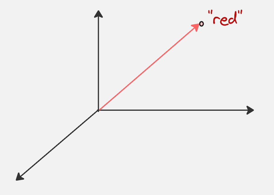
Step 2: Create Embeddings

Next, we create embeddings for our tokens. There are two types of embeddings - position embeddings and token embeddings.

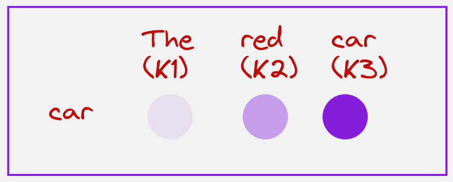
For example, if we consider the token “red”, after applying the embedding transformation, it might look as follows (we are assuming an embedding dimension of 3):

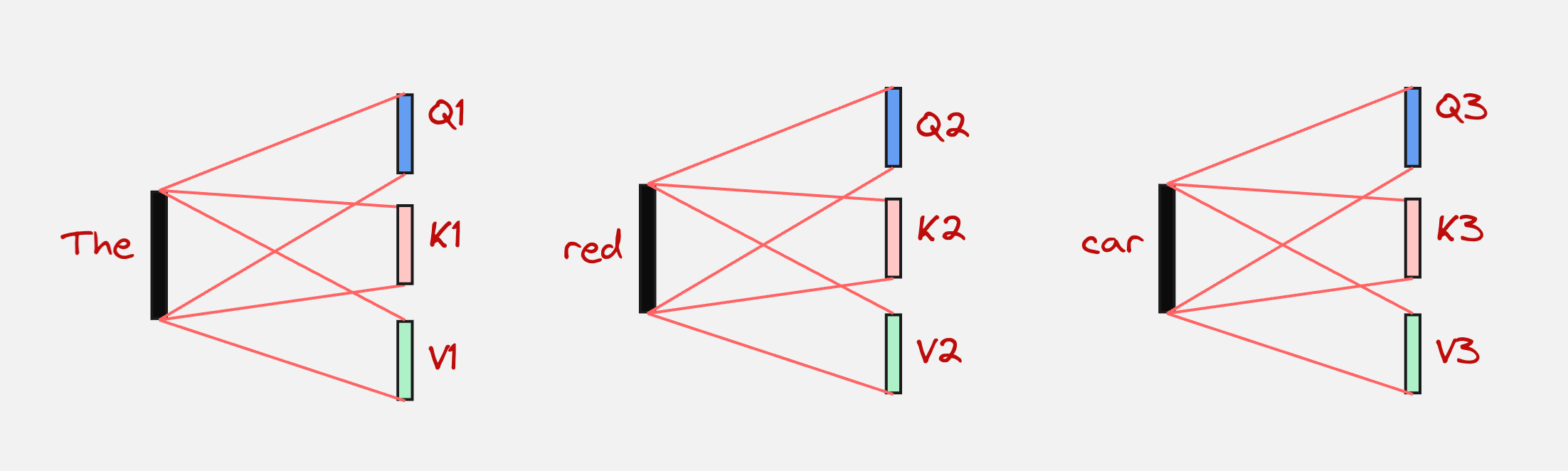
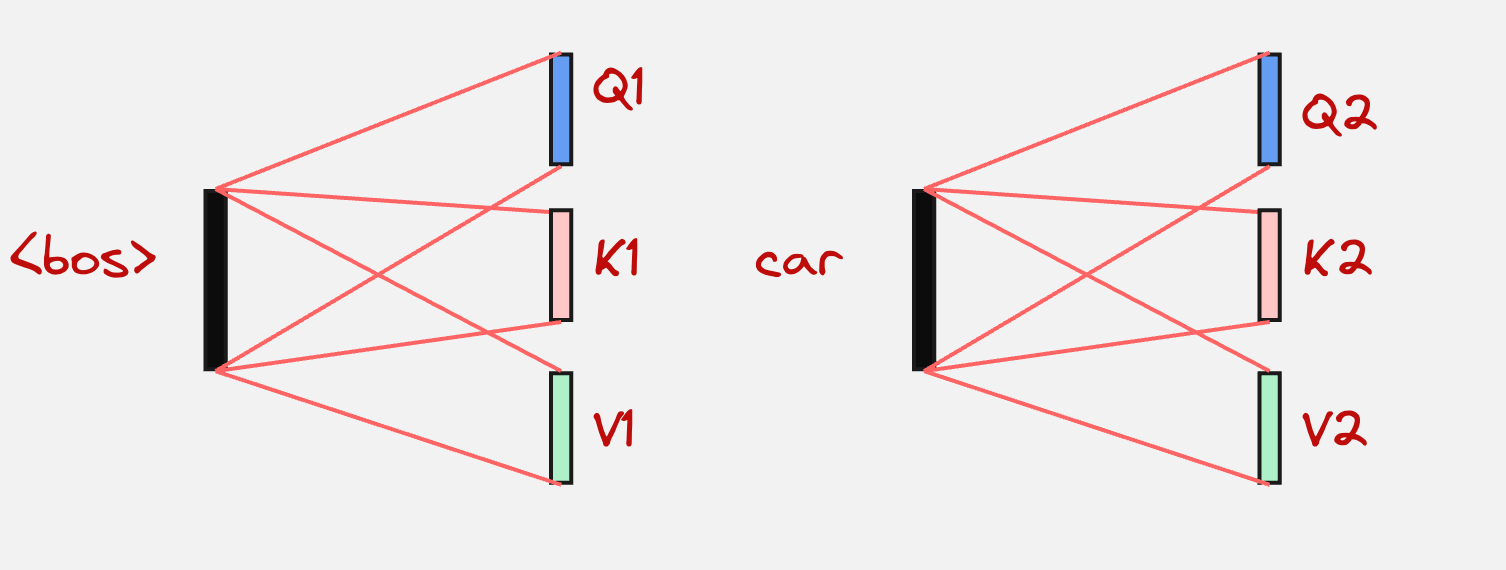
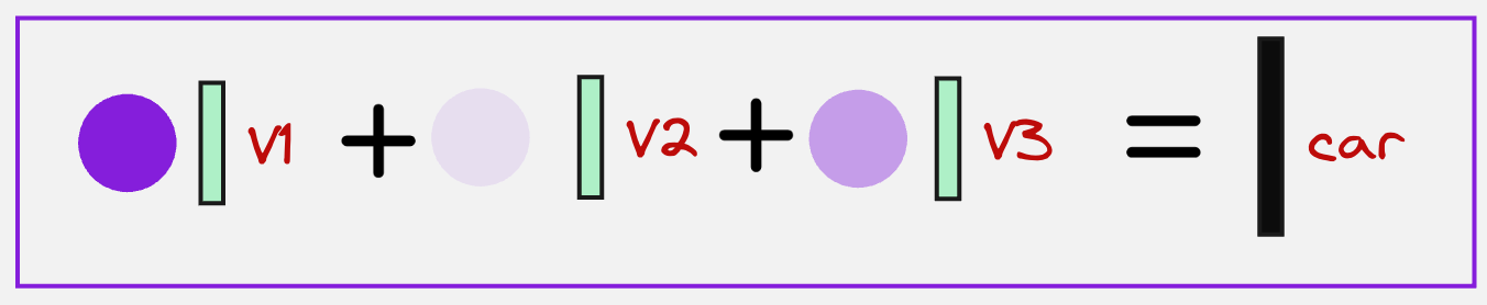
Step 3: Convert each embeddings to queries, keys and values

Every embedding is converted to queries, keys, and values. This can be represented visually as follows:

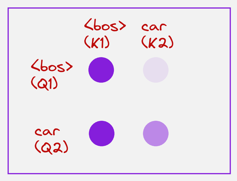
Step 4: Calculate the attention matrix

We can represent the attention matrix schematically as follows:

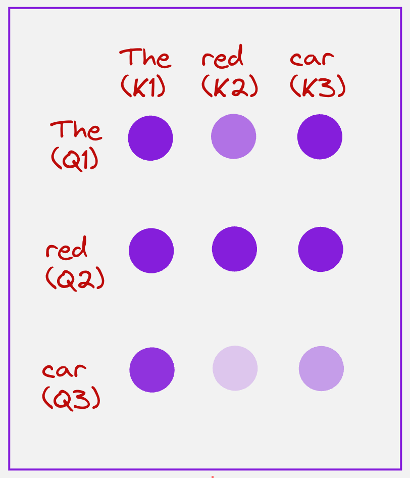
The color of the circle represents the magnitude of the attention scores. So, a brighter color means a larger attention score, and a lighter color means a lower attention score. These values lie between 0 and 1.

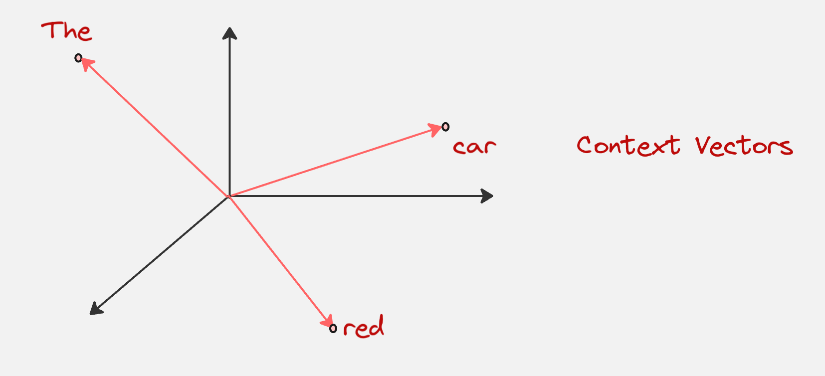
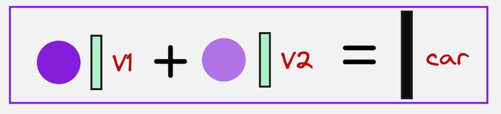
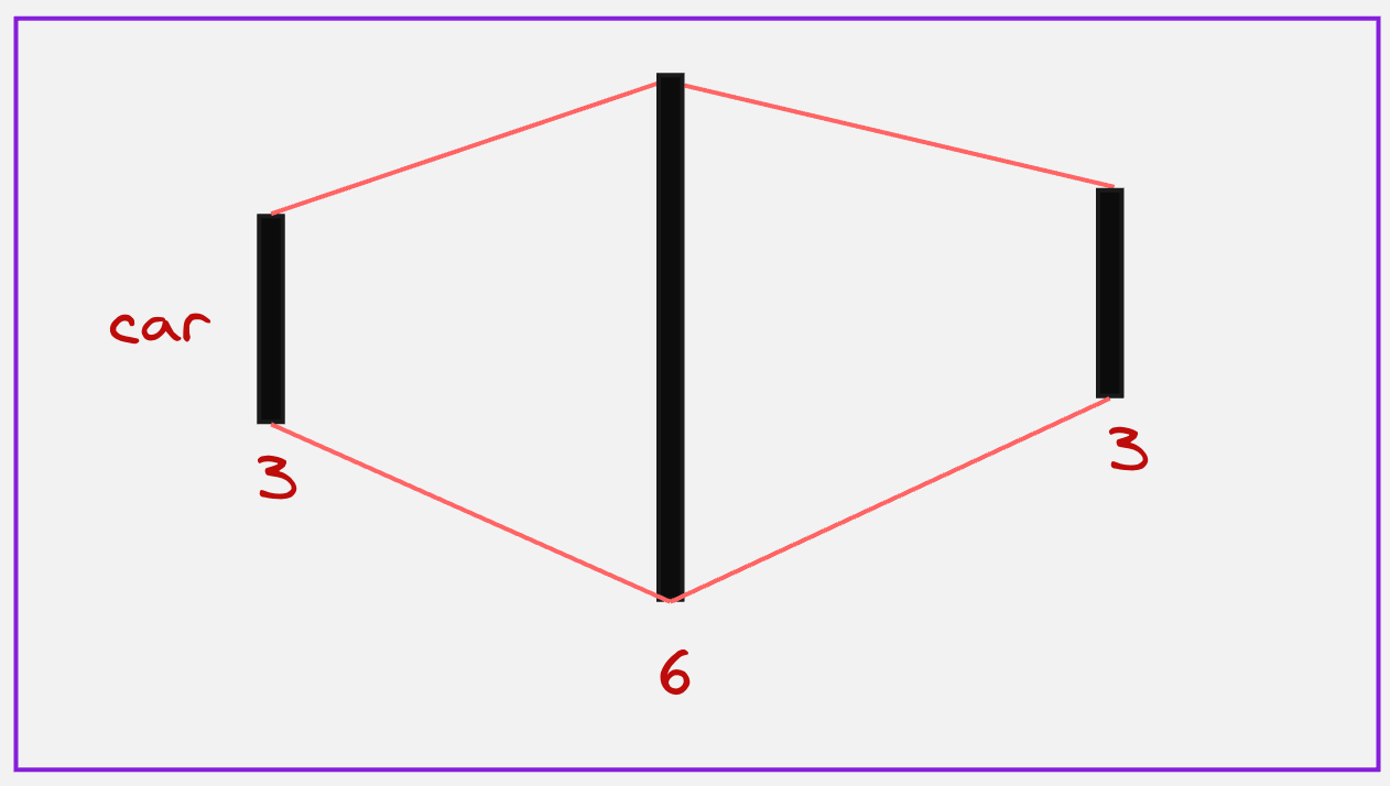
Step 5: Getting the context vectors

Once we have obtained the attention scores, we can now combine them with the values for all the tokens to get the context vector representing each token.

This can be represented schematically as follows:

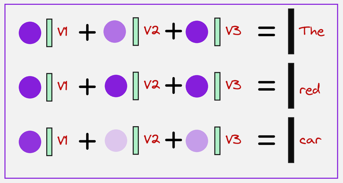
Observe what we are doing here very closely. For the token corresponding to the word “The,” we are adding all the attention values corresponding to the query “The”, and then multiplying each of them with the value vectors.

The final context vectors for all the tokens would look visually as something as follows (assuming the dimension is three):

Step 6: Passing the context vectors to the Feed-Forward Neural Network

In the next step, we pass all these context vectors to a feed-forward neural network which first increases the dimensions of these vectors and then again brings it down.

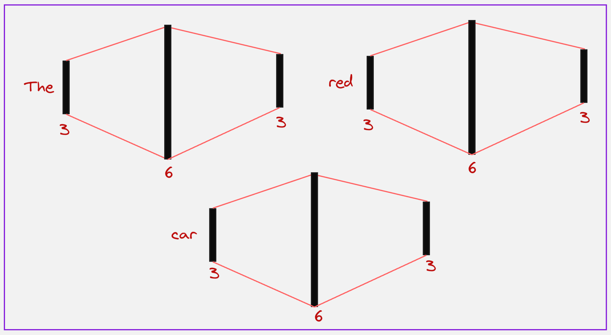
We can see here that first we increase the dimensions for all the tokens to 6, and then again bring them down to 3.

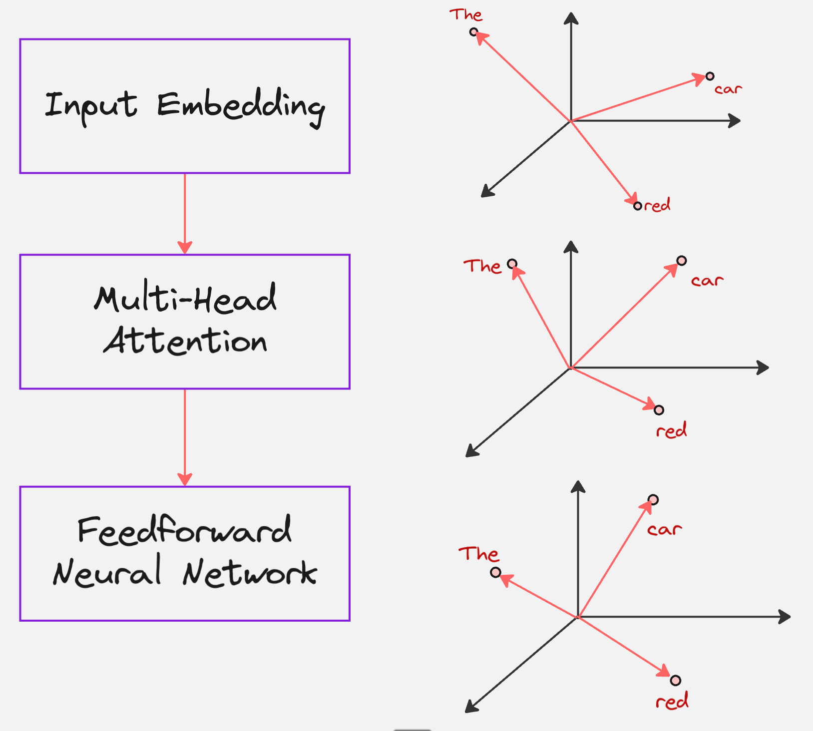
Here is how we can visualize these steps in a single diagram:

What we have until now is the Transformer Encoder. The goal of the Encoder is to read the source sentence (red car) and create a rich numerical representation of it, that understands the context of each word.

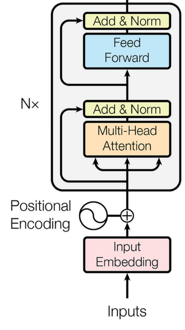
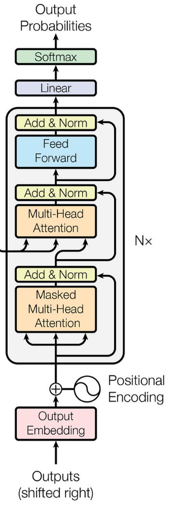
In the paper “Attention is All You Need”, which introduced Transformers to the world, they used the following schematic to represent the encoder:

But just encoding the sentences is not enough, we need something which gives us the desired output: “Swapping the adjective and noun”, in our case.

Which brings us to the Transformer Decoder.

Transformer Decoder

Let us say the input to the decoder is the following:

<bos> car

We know that the next word it should predict it red, because we want to swap the input (red car).

Step 1: Self Attention

In this step, every token in the input sequence attends to itself.

First, we calculate the query, keys and values for all tokens:

The next step is to calculate the attention matrix:

Then we find the context vector for the “car” token by using its attention values and multiplying them by the value vectors:

We have already seen these steps in the Transformer Encoder.

After this comes a very unique step, which is called “cross-attention”

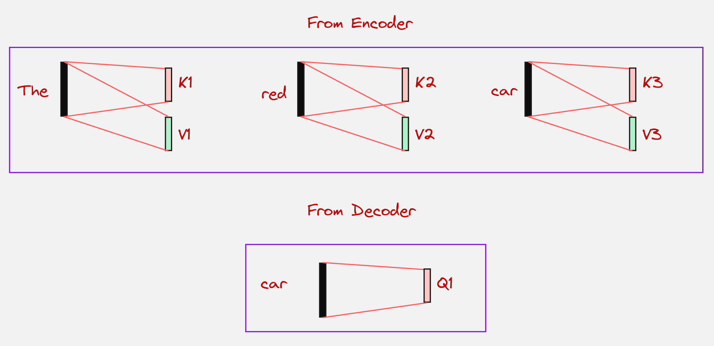
Step 2: Cross-Attention

In the cross-attention layer, the query comes from the decoder side, but the keys and values come from the encoder side.

In the above example, we will use the context vector for the “car” token to calculate the query, but the keys and values will come from the encoder. Let us look at the visualization below to understand this:

Once the query, keys and values have been computed, we can calculate the attention scores:

Note that here we are trying to understand how much the token “car” relates to all the tokens in the input sentence. This is important for us because we know that the attention score for the token “red” is going to be high, since we want to swap the adjective and the nouns.

After this, we again calculate the context vector in a similar fashion like we have done a couple of times before:

Note that here the values are coming from the encoder tokens.

You might have guessed what happens next. We pass it through the feed-forward network, just as we did with the encoder, where we increase the dimensions and then decrease them again:

The Decoder’s job is to generate the translation one word at a time, using the memory created by the Encoder.

What next? How do we generate the next token?

One last step is remaining:

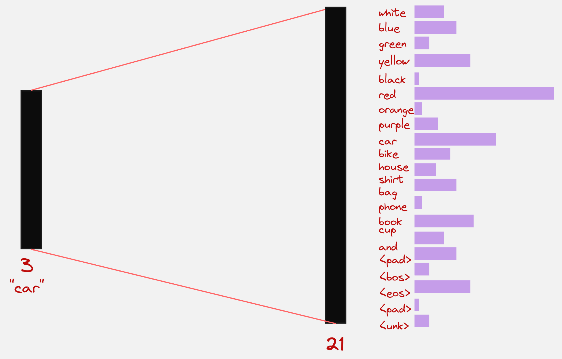
Step 3: Projection into the Vocabulary Space

In this step, what we do is, we take the context vector from the previous step and then we project it into the entire vocabulary space. We look at which token has the maximum value, and we choose that as our next token. This can be visually presented as follows:

In the paper “Attention is All You Need”, which introduced Transformers to the world, they used the following schematic to represent the decoder:

We have explained the example which we started out with from scratch in a Google Colab notebook which you can use to understand the entire architecture. Here is a link to the notebook:

Google Colab Notebook: Designing Transformer Encoder and Decoder for Swapping Adjective and Nouns

Here is the sample output which we get:

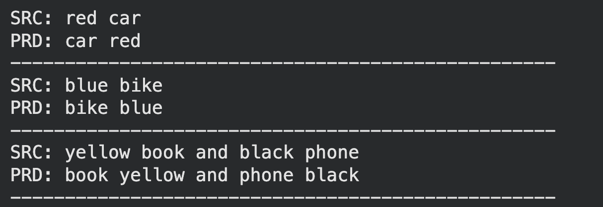
Hmm..Not bad!

In the field of robotics, we will be mostly working with image-based data.

We should develop a method which can look at images and understand the context from the images.

This brings us to the topic of vision transformers.

Vision Transformers:

Let us understand what happens inside a Vision Transformer:

We will take an example of one of the observations collected from our robot (we use an SO-101 Robot in our company). Let us say the observation looks as follows:

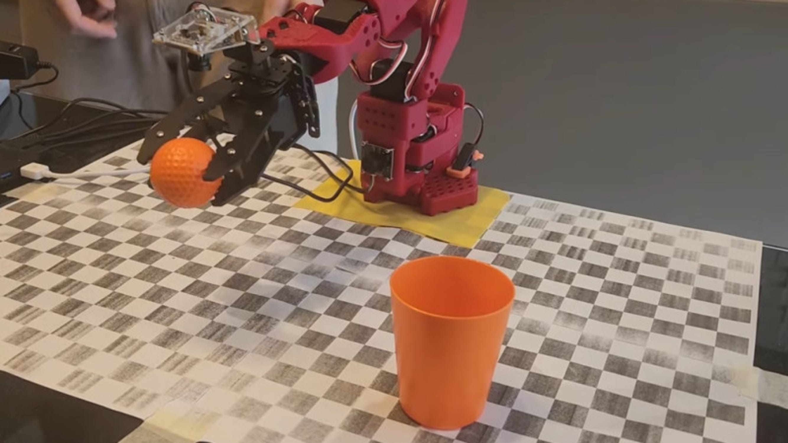
From this image, we can probably guess that the camera is mounted somewhere in front of the robotic arm, and the task that the robot is trying to perform is to place the golf ball into the orange cup.

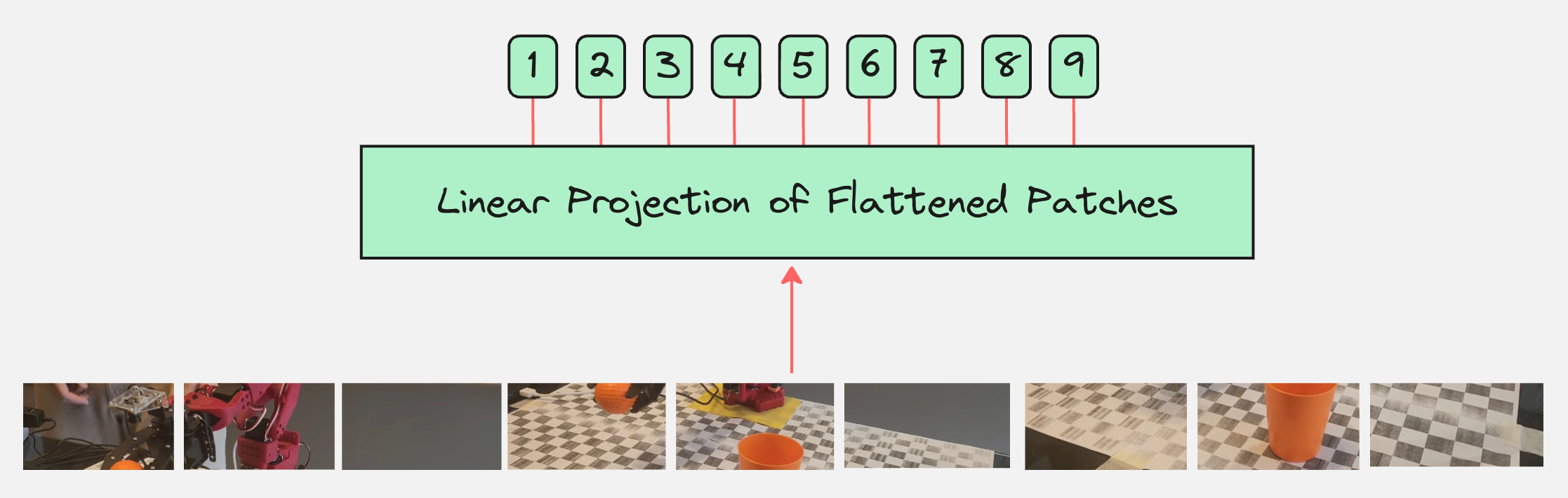
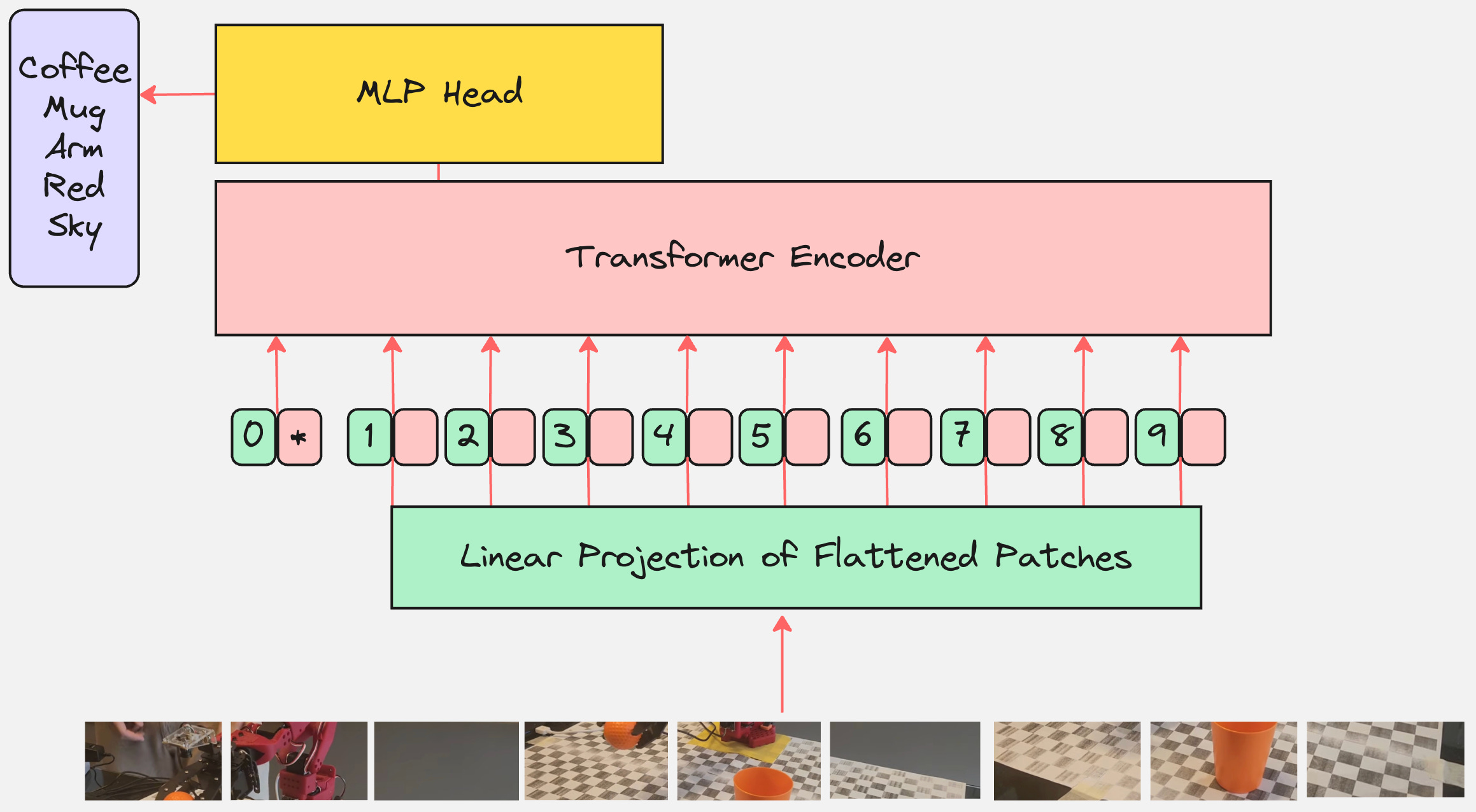
Step 1: Dividing the image into patches

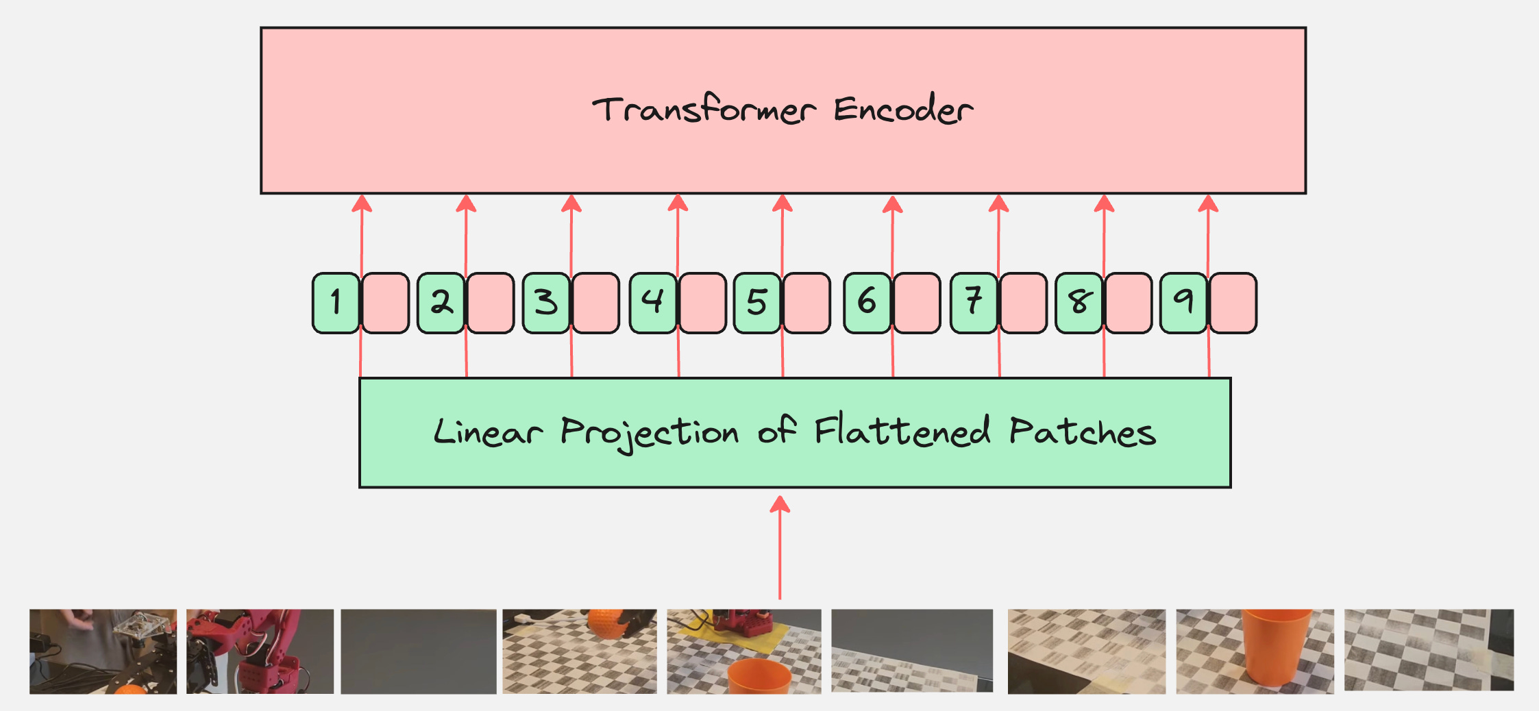
In the first step, we will take the image and divide it into a specific number of patches. Let us visually see how this looks like for the above observation:

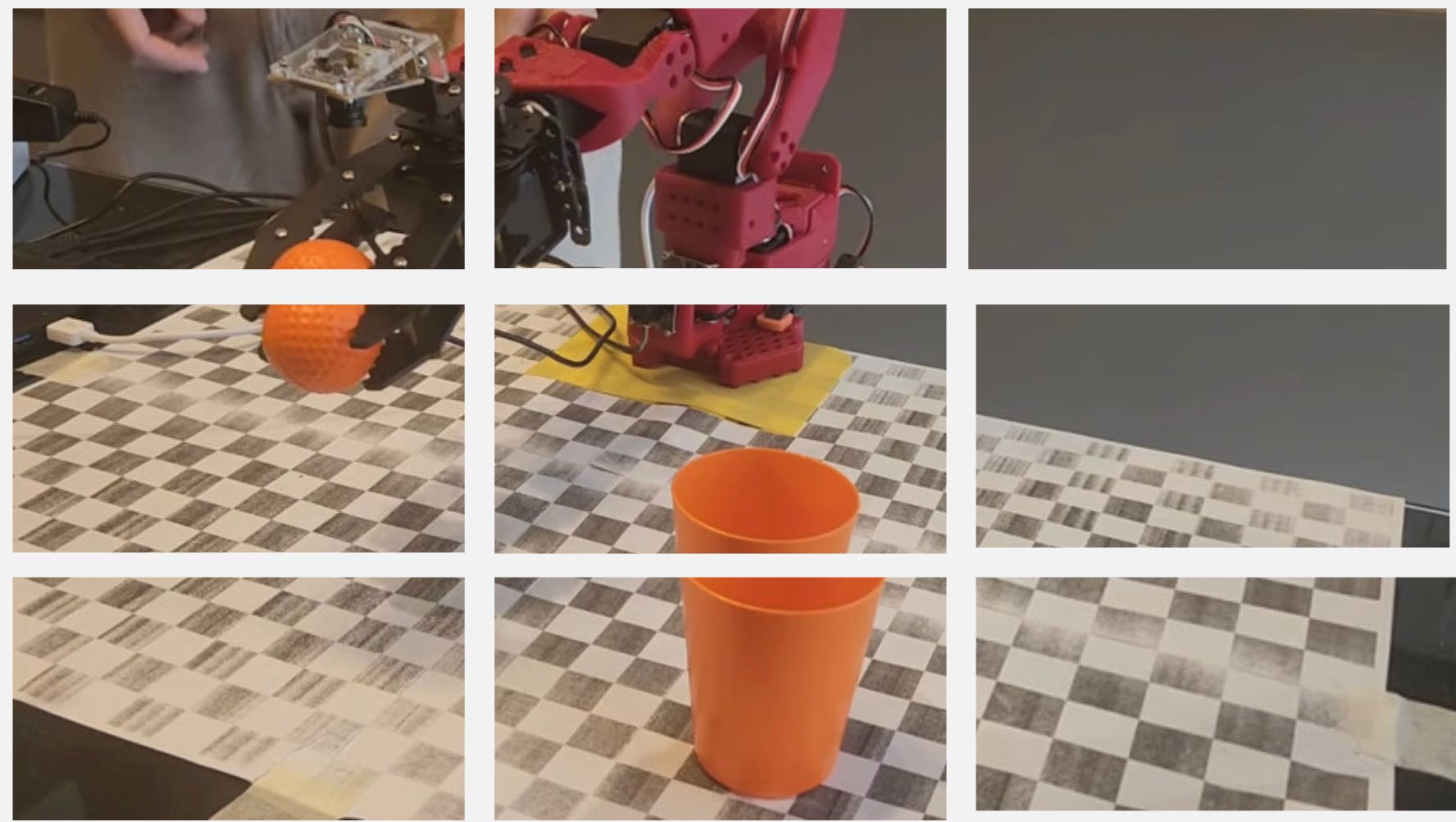
Okay, we have divided the image into 9 patches, what next?

Remember that in the transformer architecture, which we discussed before, we had a layer that converted the token into token embeddings.

But we do not have tokens here. So, what do we do instead?

What if we take the patches and convert them to patch embeddings?

Let us look at how exactly patch embeddings are created

Step 2: Creating Patch Embeddings

Let us say the dimensions for each of our patches is 28x28x3, so totally we have 2352 values.

Now imagine a neural network which takes these 2352 values as an input and produces an output of dimension 512.

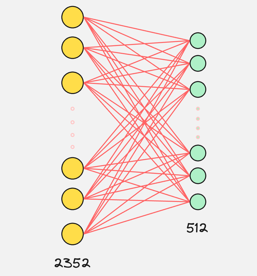
This is what is visually happening in the creation of the patch embeddings.

So, the process till now can be visually represented as follows:

This looks good for now, but we are forgetting something!

Step 3: Creating Position Embeddings

Imagine that you have the following pictures:

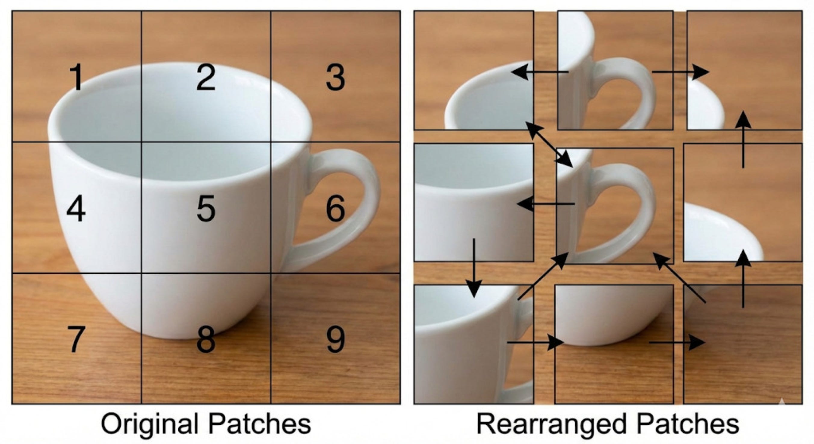
Both the images contain the same patches. The only difference is that they are rearranged.

Now, if we continue with the above architecture, our model would treat both these images as the same. It would not understand the importance of the ordering of the patches inside these images.

This is why, along with patch embeddings, we need position embeddings as well.

We had done the same thing for the Transformer architecture when applied to language data, where the position embeddings were calculated for the tokens that come in a sequence.

When we add the position embeddings, our modified architecture looks as follows:

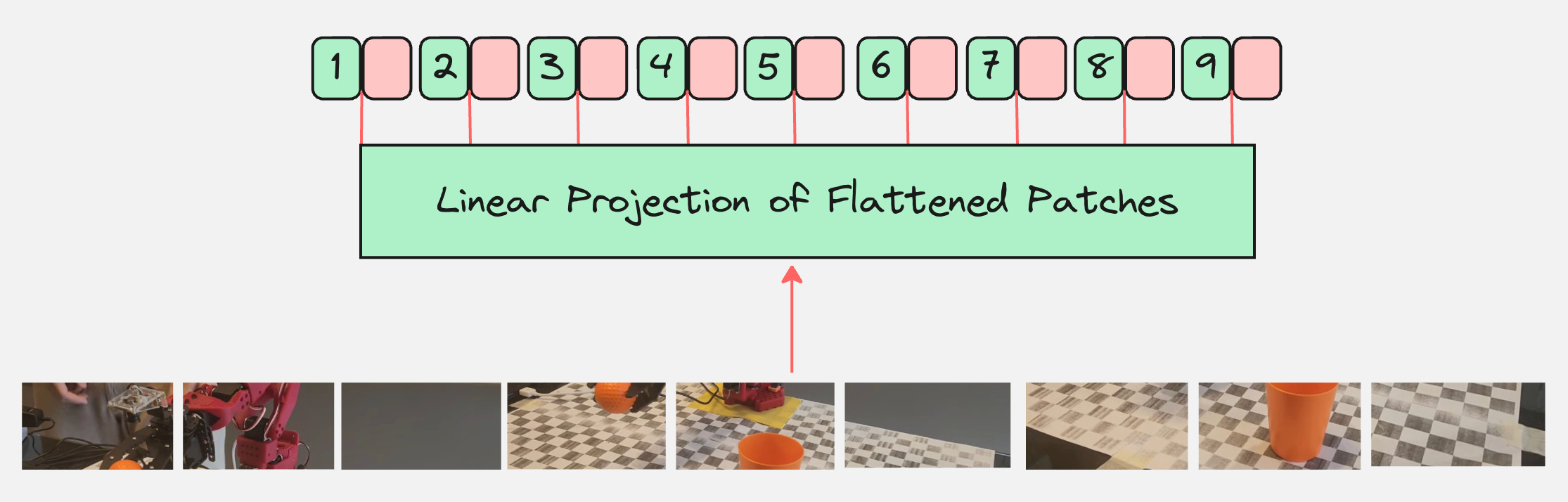
Now, we simply pass this as an input to the transformer encoder.

Step 4: Pass this as an input to Transformer Encoder

Are we done?

Question: What is the output of the transformer encoder?

How do we use it to classify the images?

Remember that the output of the transformer encoder are the context vectors for all tokens.

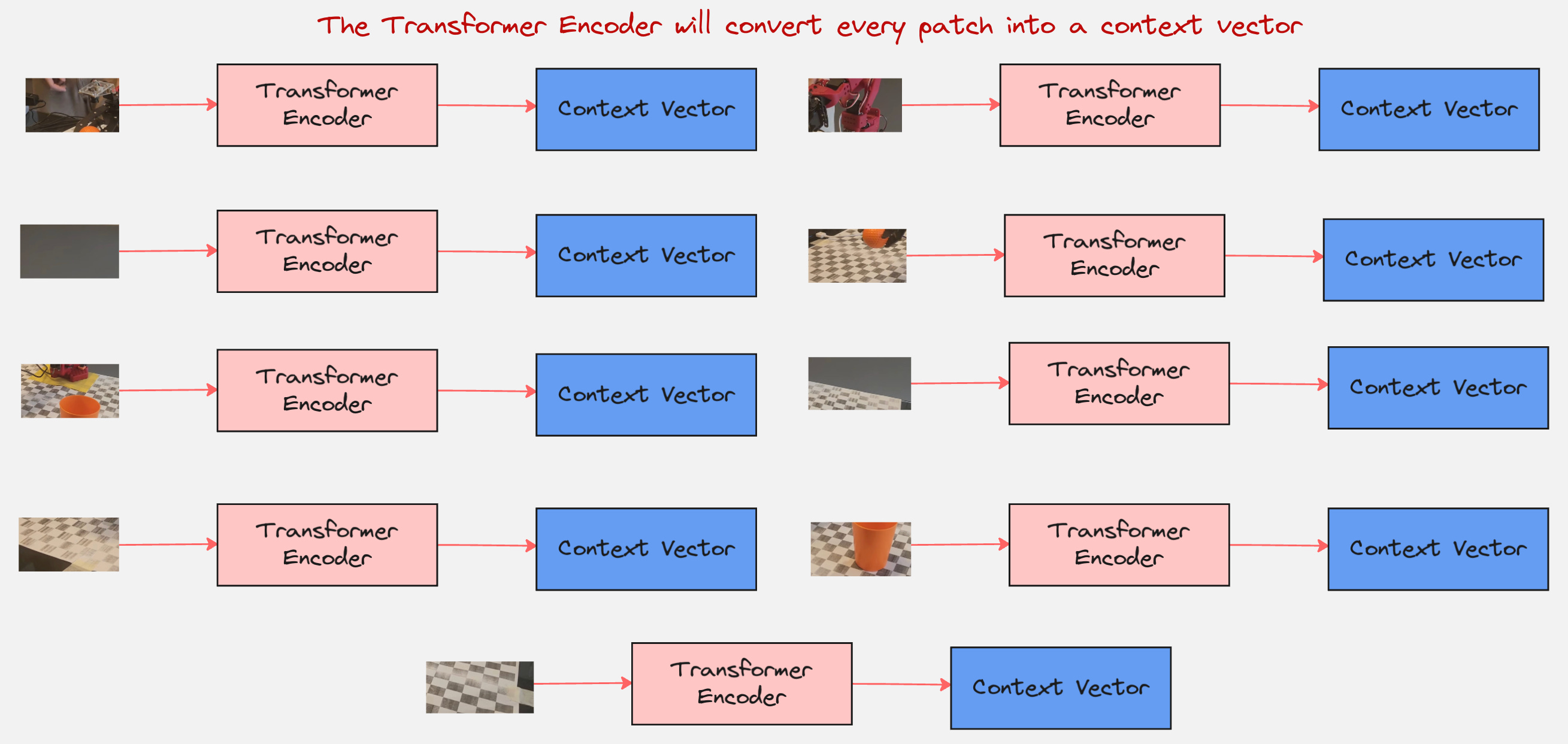
So, what next? How do we classify this image?

This is where we come to an important concept.

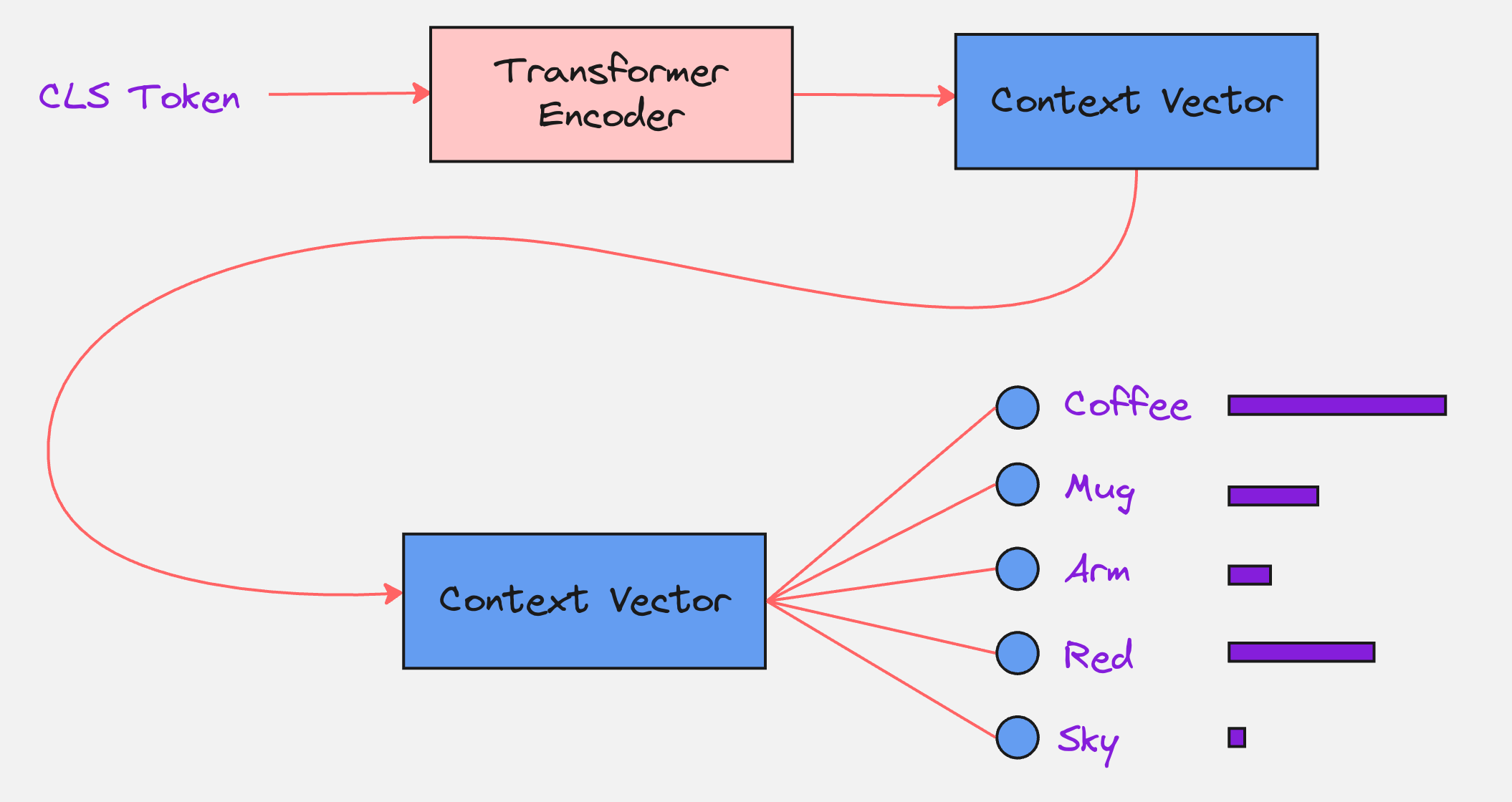
Step 5: Classification Token [CLS]

We add a learnable embedding to the sequence of embedded patches whose state at the output of the Transformer encoder serves as the image representation.

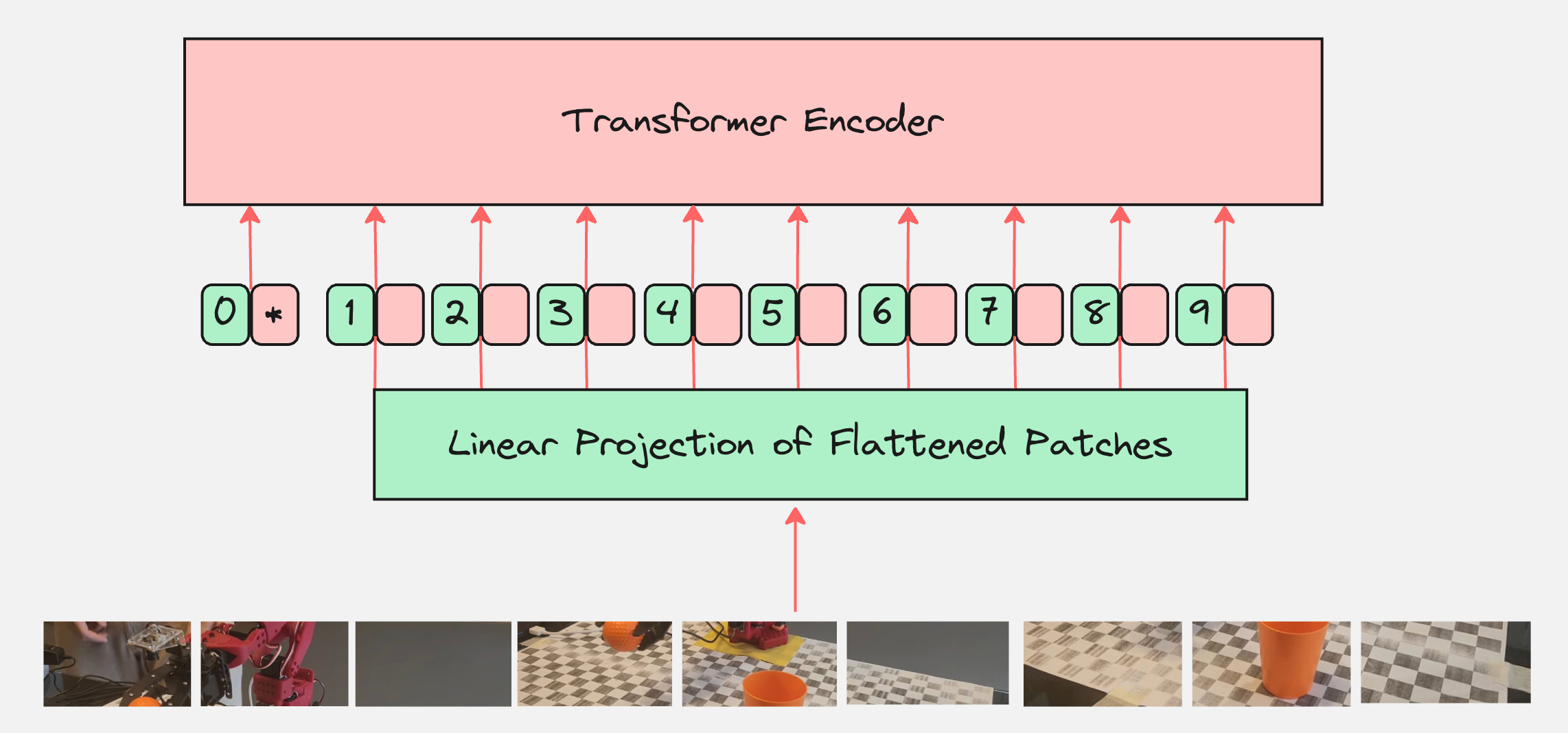
This learnable token is also called the “class” token or the “classification” token.

To understand what the CLS token does, let us calculate the attention matrix and the role of this token in the attention matrix.

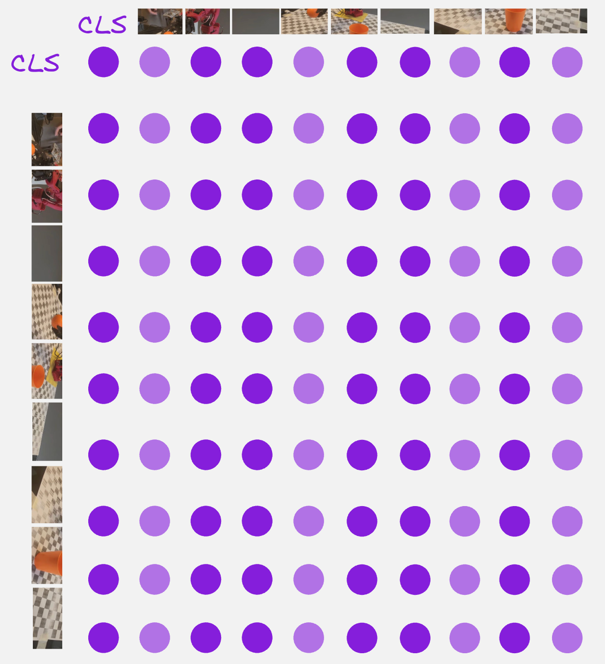
From the above attention matrix, we can see that the CLS token is attending to itself and also the other 9 patches.

So, the CLS token can be thought of as something which contains a summary of the entire image.

Question: Can we think of how do we move from here to how the context vector is generated for the CLS token?

This brings us to the next step:

Step 6: The Classification Head

The last step is the classification head. Here, the context vector corresponding to the CLS token is passed through a multi-layer perceptron with the output dimensions which are equal to that of the number of classes which we have.

The final Vision Transformer Architecture looks as follows:

Let us look at a practical example to understand how ViT is implemented in practice:

We will look at the following dataset:

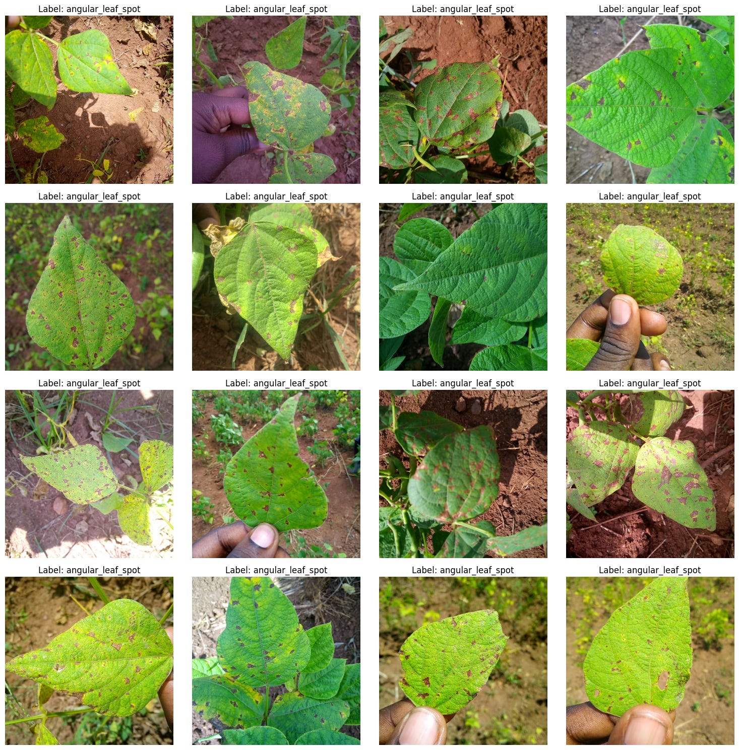
There are 3 classes here:

(1) angular_leaf_spot (A fungal disease causing angular spots on leaves)

(2) bean_rust (A fungal disease causing rust-colored pustules)

(3) healthy (No disease detected)

We will use a pretrained Vision Transformer as our base model and then fine-tune it for our specific task.

We will use the following Transformer:

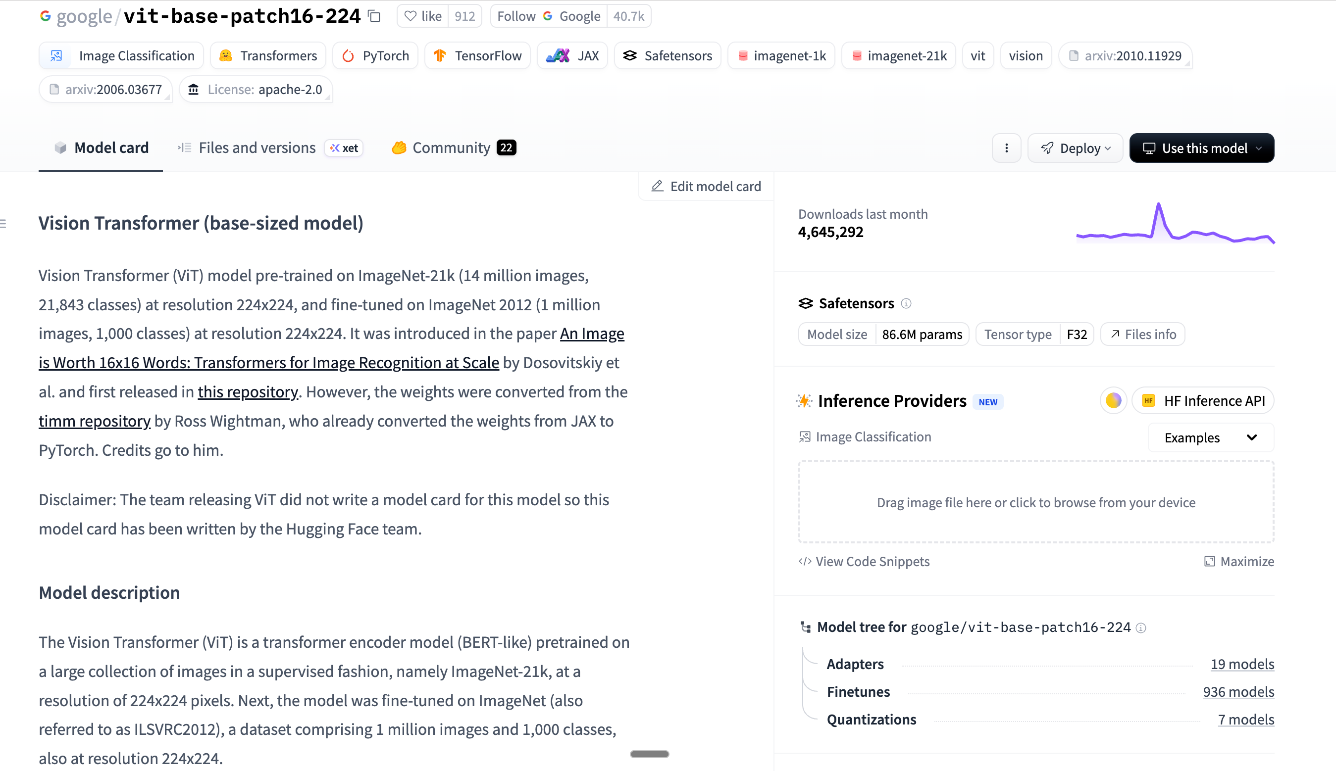
This model was pretrained on a large collection of images in a supervised fashion, namely ImageNet-21k, at a resolution of 224x224 pixels. Next, the model was fine-tuned on ImageNet (also referred to as ILSVRC2012), a dataset comprising 1 million images and 1,000 classes, also at resolution 224x224.

We use the following pipeline for our task:

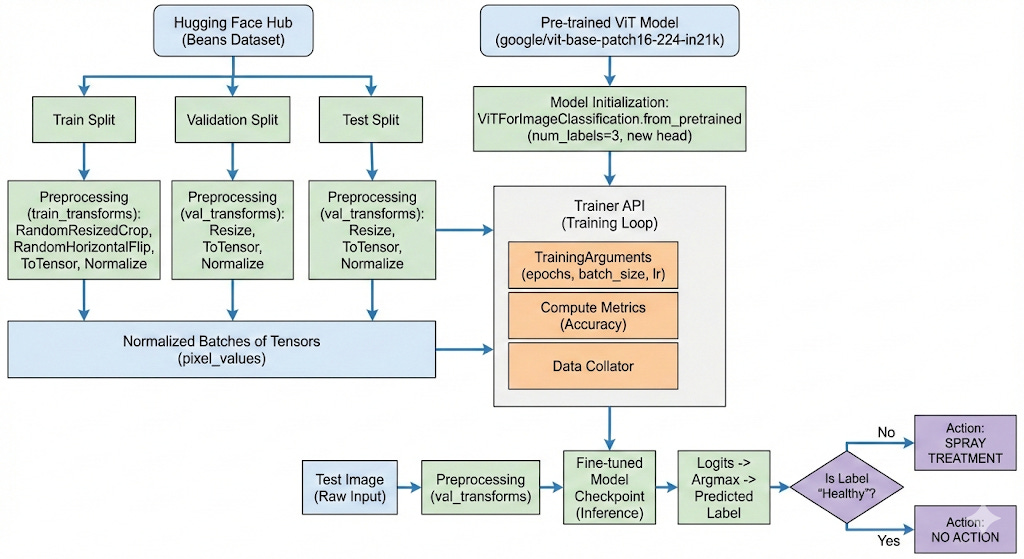
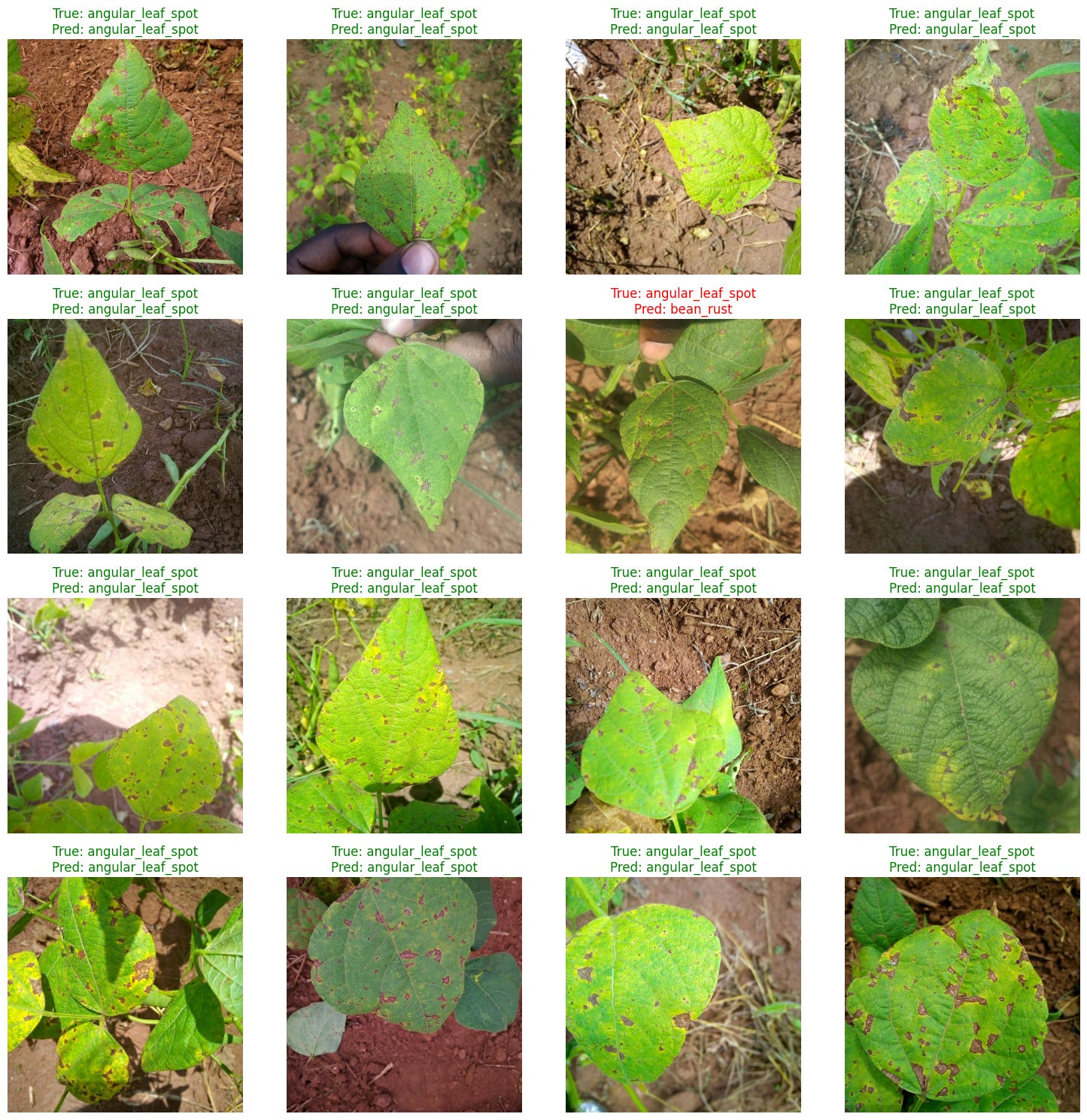
After training for 3 epochs, we get an accuracy of 96%. See the result below:

Here is the link to the Google Colab Notebook:

Google Colab Notebook: Implementing Vision Transformer on a Practical Dataset

Here is the link to the original paper which introduced Transformers: https://arxiv.org/abs/1706.03762

Here is the link to the original paper which introduced Vision Transformers: https://arxiv.org/pdf/2010.11929

If you like this content, please check out our bootcamps on the following topics:

Modern Robot Learning: https://robotlearningbootcamp.vizuara.ai/

GenAI: https://flyvidesh.online/gen-ai-professional-bootcamp

RL: https://rlresearcherbootcamp.vizuara.ai/

SciML: https://flyvidesh.online/ml-bootcamp

ML-DL: https://flyvidesh.online/ml-dl-bootcamp

CV: https://cvresearchbootcamp.vizuara.ai/