The Journey of a Single Token
Introduction to transformer architecture


When people look at the transformer architecture for the first time, what they usually see is a dense diagram filled with blocks, arrows, and unfamiliar terms. It can feel overwhelming, like trying to understand a machine by staring at its circuit board. A more intuitive way to approach it is to trace the journey of a single token as it travels through the architecture. What happens to that token at each stage? How does it change shape, meaning, and numerical representation? This narrative gives us a much clearer sense of why the transformer works the way it does.
From Words to Numbers
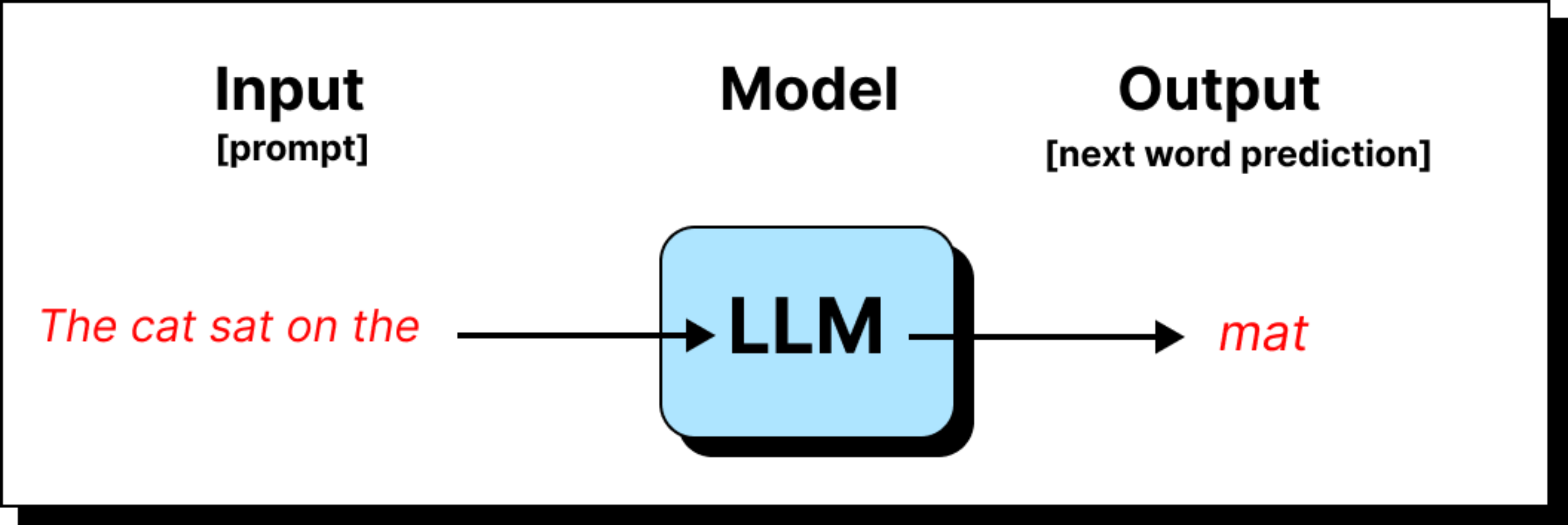
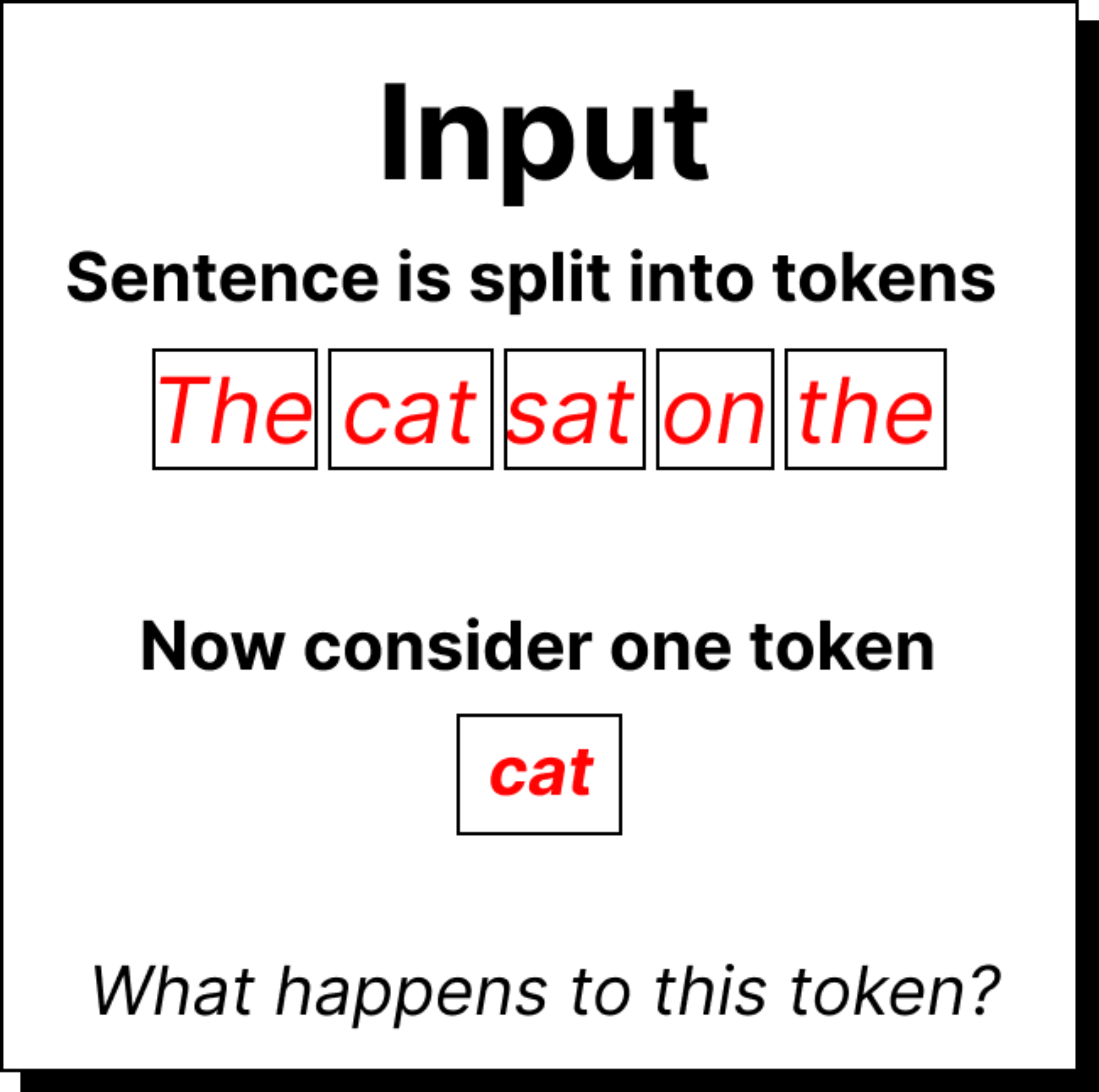
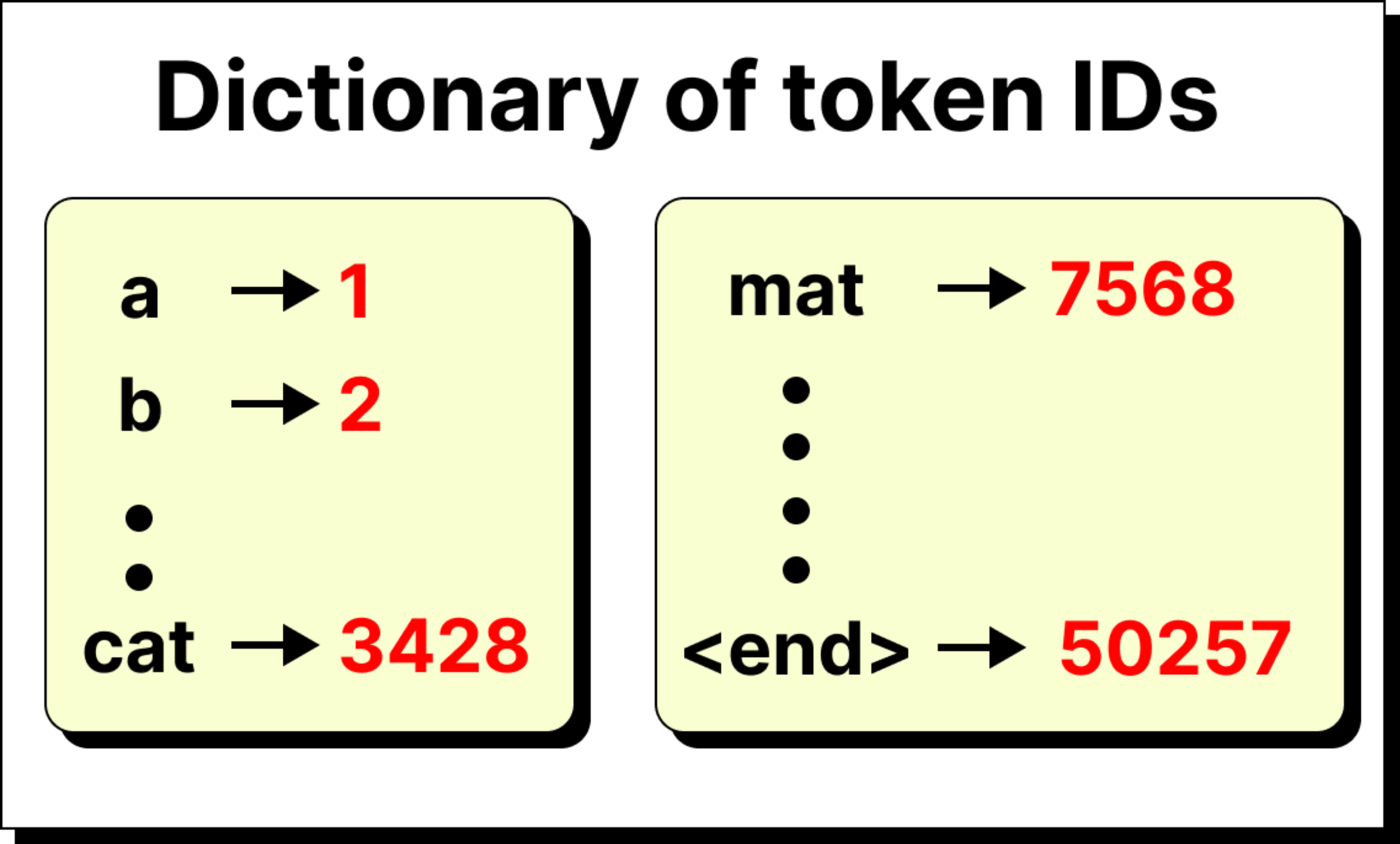
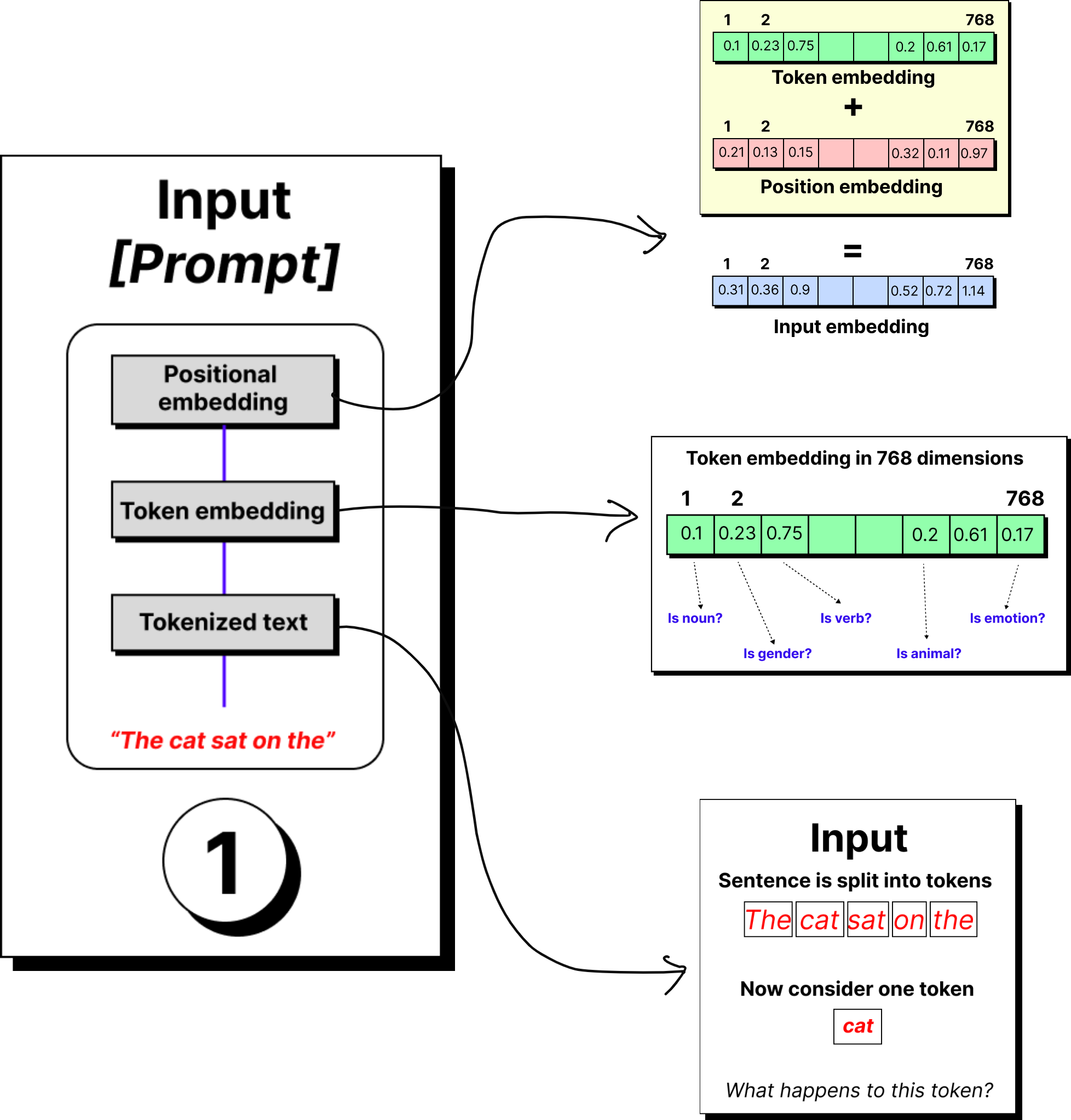
The story begins with the tokenizer. A sentence like the cat sat on the mat is broken down into tokens. These tokens may be entire words, or more often, sub-words and fragments, depending on the vocabulary of the model. Each token is then mapped to a unique numerical identifier from a fixed dictionary.
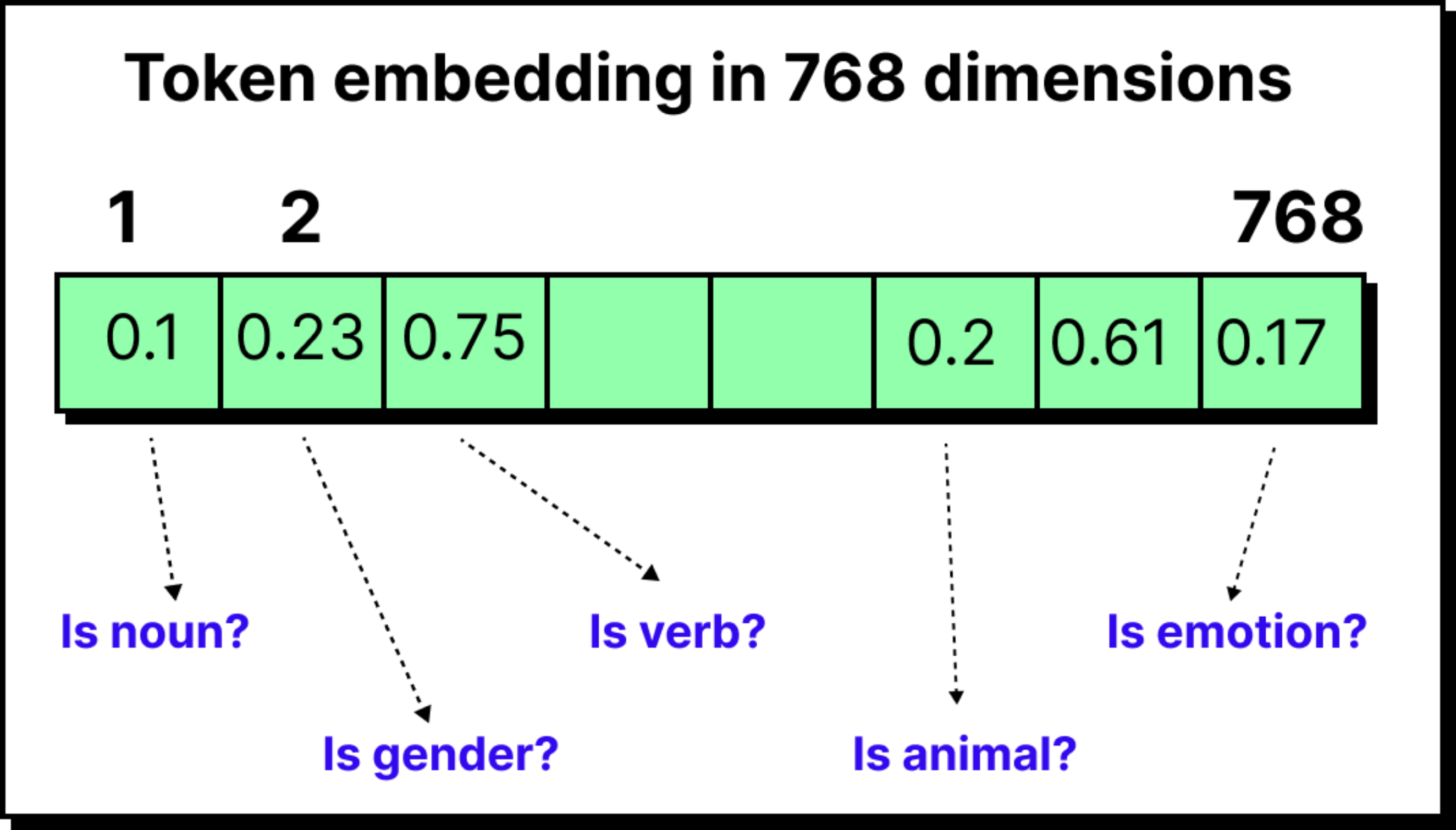
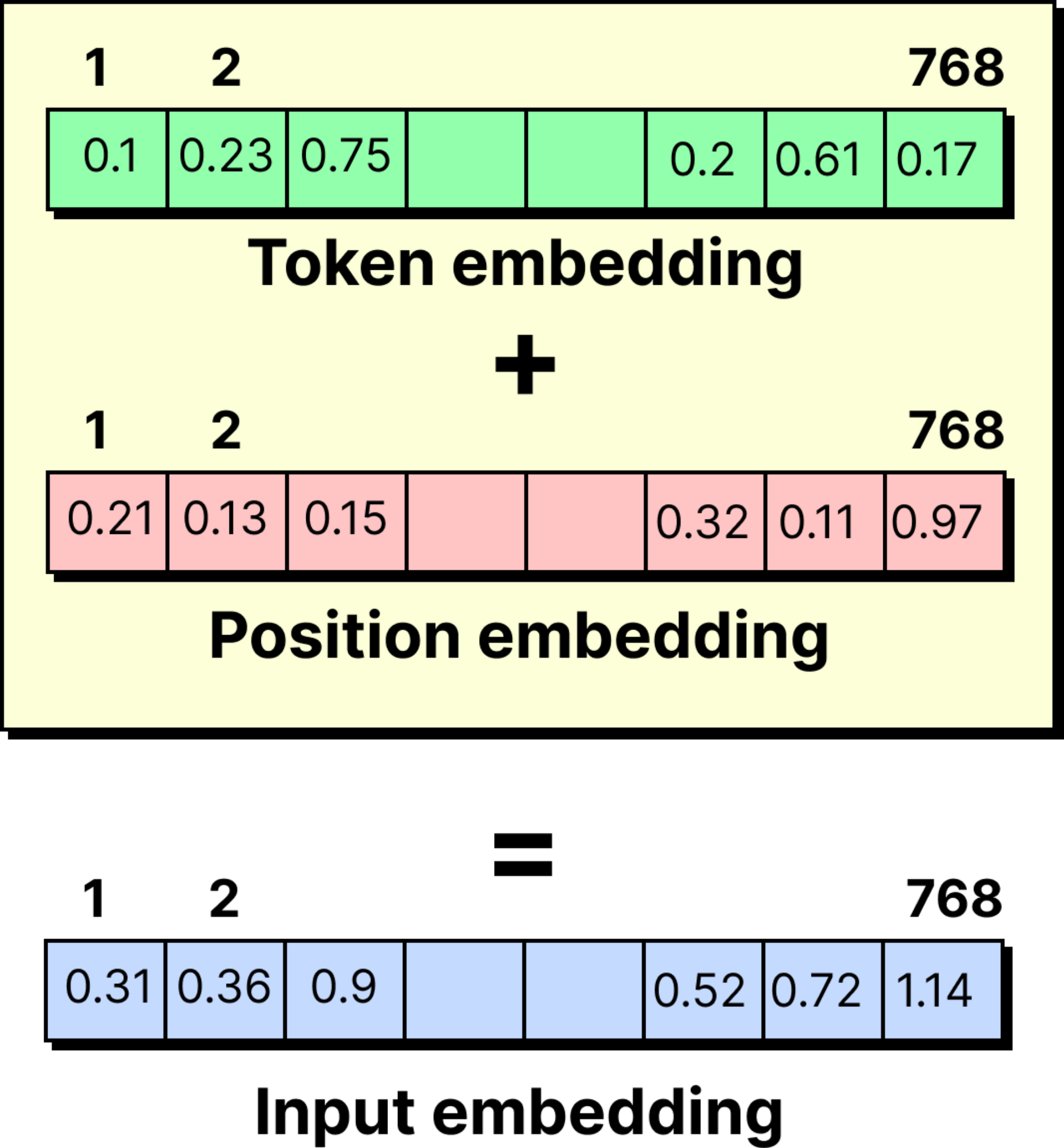
But raw IDs are not useful by themselves. The model requires vectors that capture meaning, so every token ID is passed through an embedding layer. This layer assigns a vector, for instance of 768 dimensions in GPT-2, that represents the token in a learned semantic space.
At this stage, the word cat is no longer just “cat” but a 768-dimensional fingerprint that captures how it relates to other words in the training data.
Positional Encoding
There is, however, a missing piece. A sequence of tokens must carry order. “The cat sat on the mat” is not the same as “The mat sat on the cat.” Without positional information, the embeddings look identical in both cases.

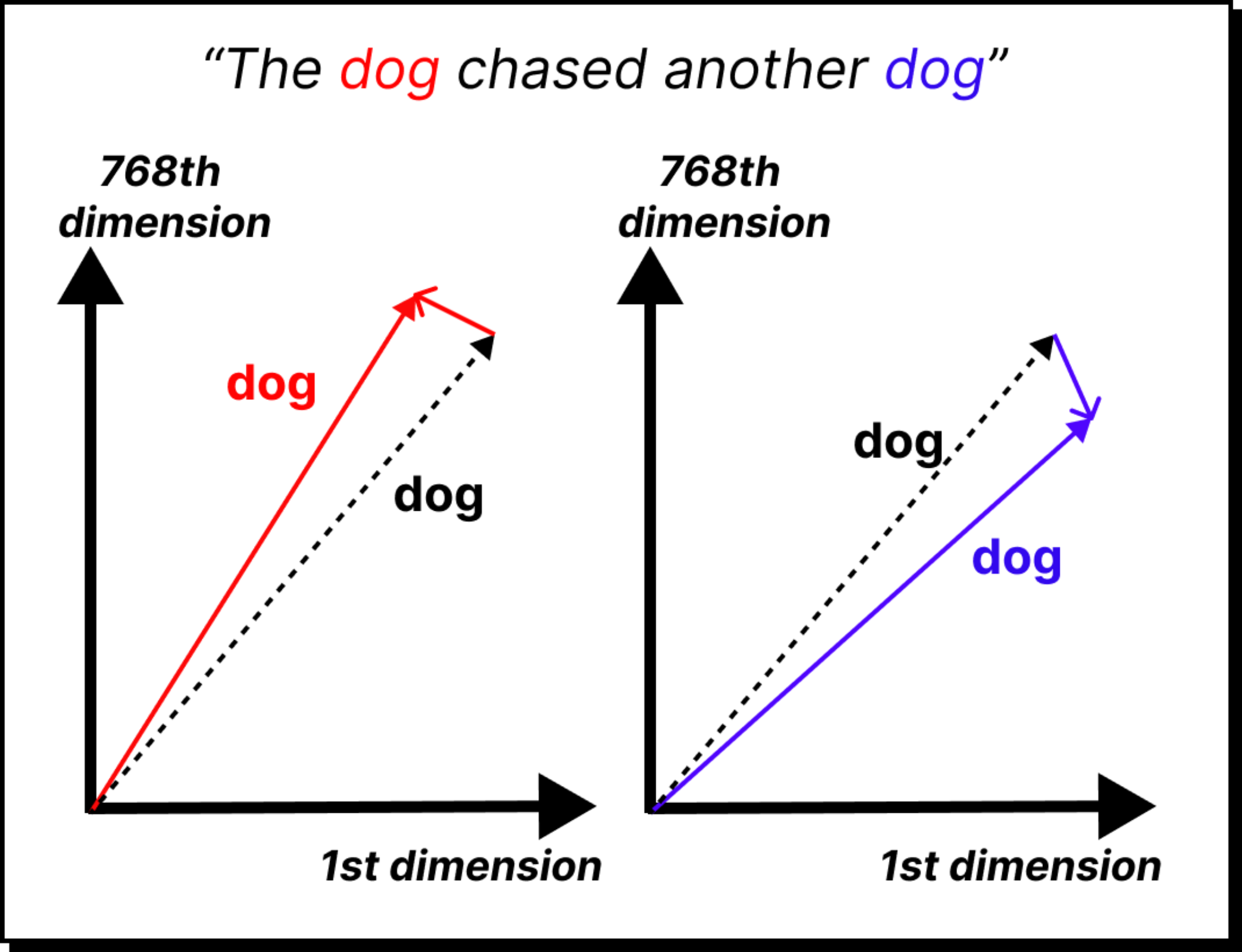
Transformers solve this problem by adding positional encodings. For every position in the sequence, a special vector is created and added to the embedding. The result is a combined representation where each token knows not only what it is, but also where it belongs. With this, cat in the second position is different from cat in the fifth position.
Entering the Transformer Block
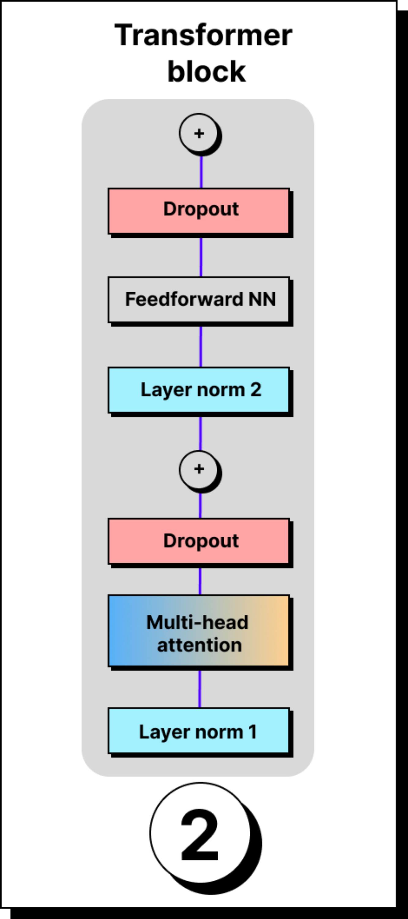
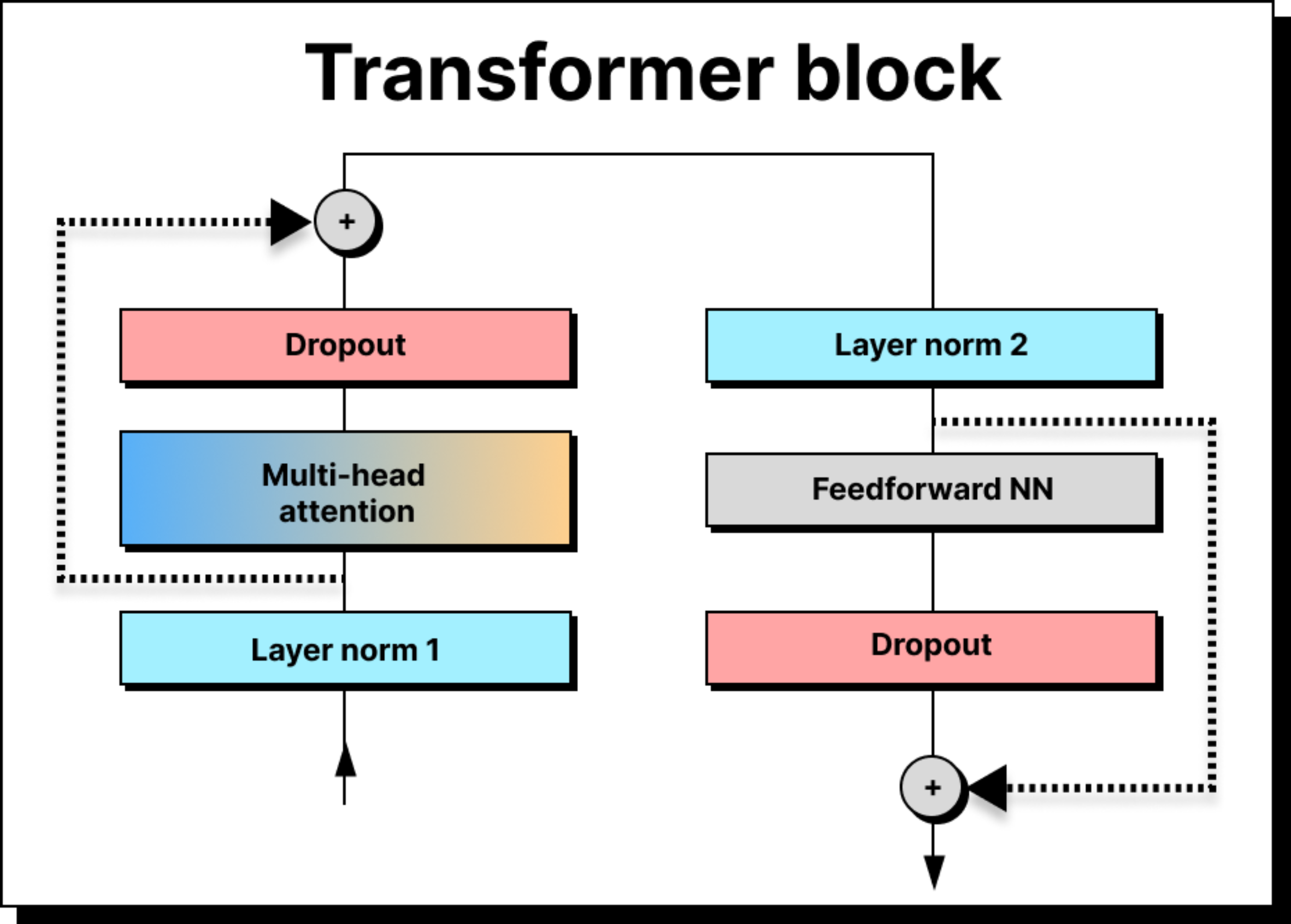
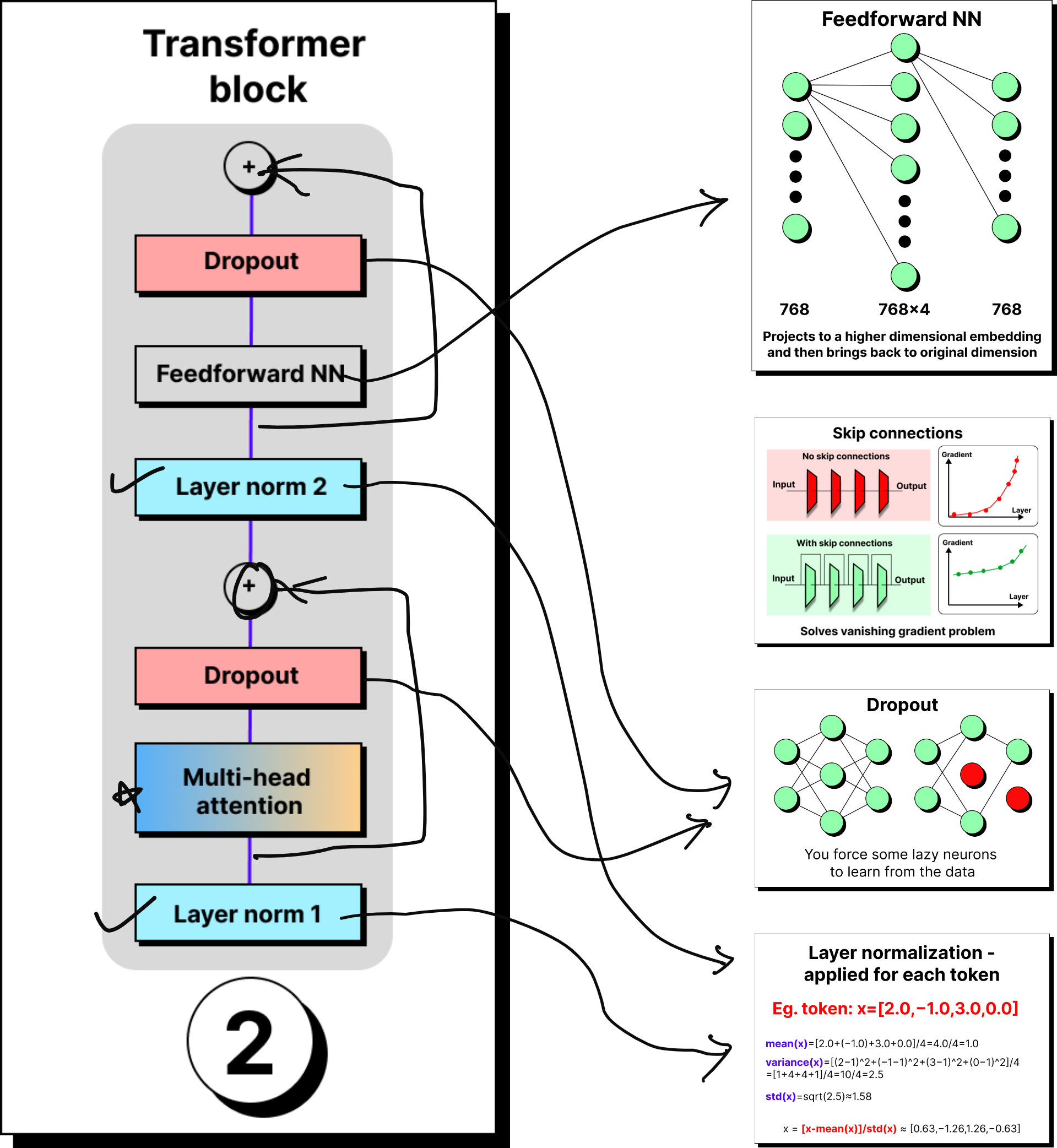
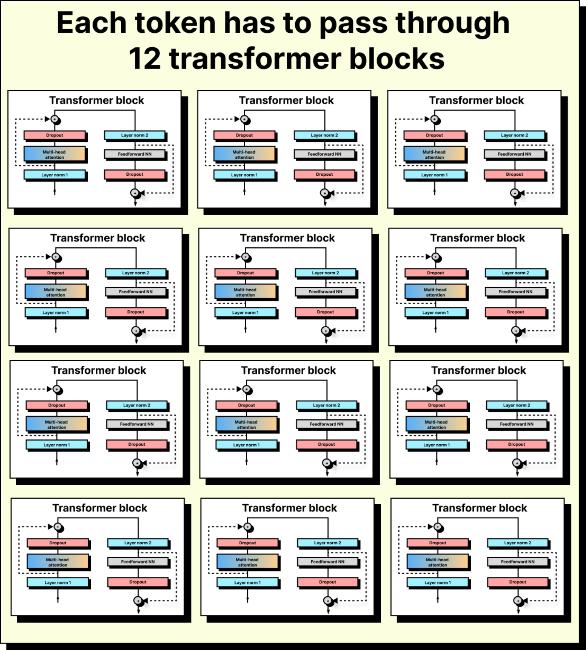
Once tokens are embedded and positionally enriched, they enter the transformer block. A transformer is not just one block, but a stack of many identical ones – 12 in GPT-2, 96 in GPT-3 – arranged in series. Each block refines the token representation further, passing it through the same set of components: layer normalization, multi-head attention, dropout, skip connections, and feed-forward networks.
Layer Normalization
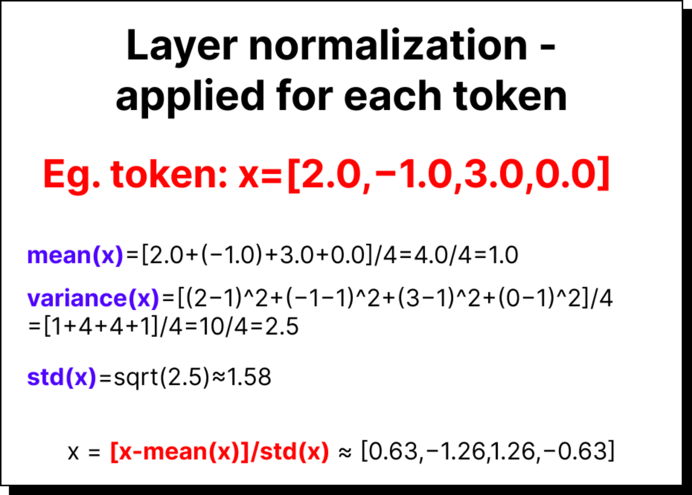
The first operation in the block is layer normalization. Here, the values of the token vector are standardized by subtracting the mean and dividing by the standard deviation. If we stopped here, the mean would always be exactly zero and the variance exactly one, which sometimes over-constrains the representation.
To allow flexibility, two trainable parameters are introduced for every dimension of the token: beta and gamma. Beta acts as a scaling factor and gamma as a bias. They begin with random values and are adjusted during training. This means that while normalization pushes values toward zero mean and unit variance, beta and gamma allow the model to reintroduce extremes where necessary. If a certain feature must have a large value to represent something meaningful, the model can learn that through these parameters.
Without beta and gamma, normalization would flatten important differences. With them, the model can stabilize training while still keeping the ability to represent nuances.
Dropout and Regularization
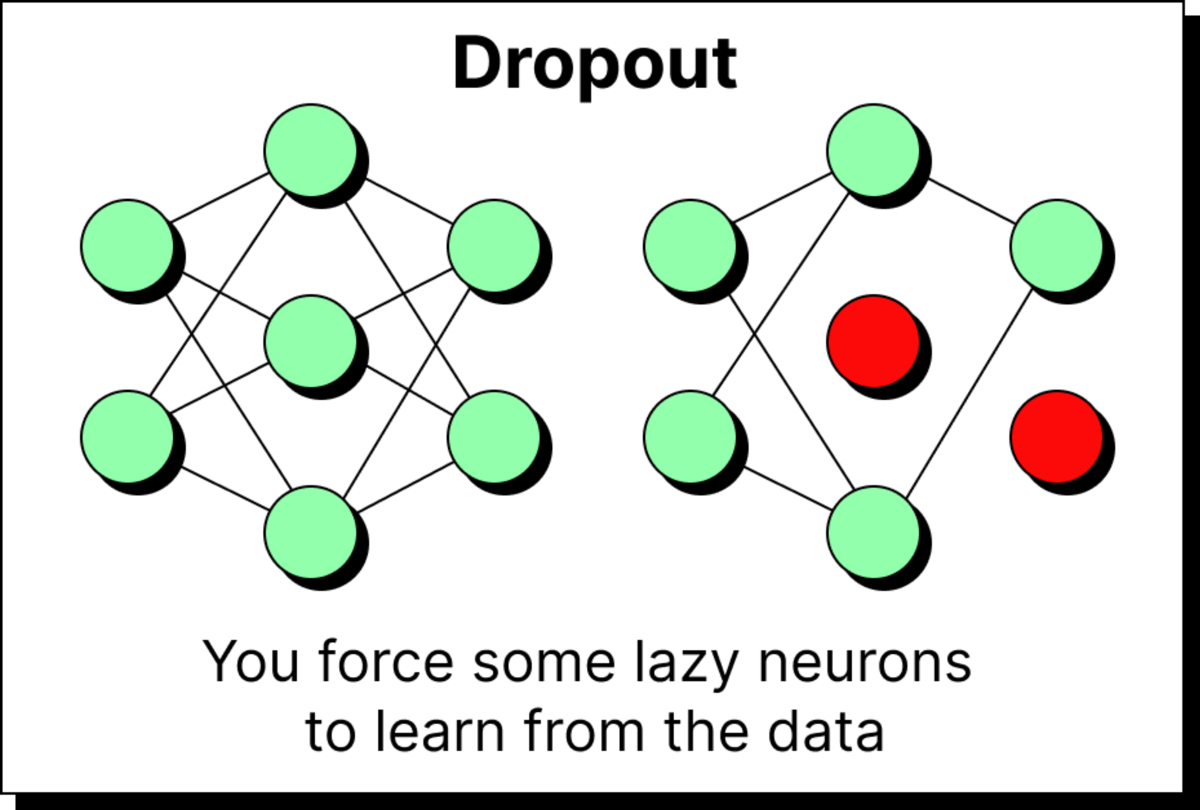
After normalization, dropout is applied as a regularization step. The idea is straightforward: during training, some neurons are randomly switched off. If all neurons participated equally in every loop, certain neurons might become lazy, letting others do the heavy lifting. Dropout prevents this by forcing the burden of learning to spread across the network.
If 20 percent of neurons are dropped in a layer, only the remaining 80 percent are active. To avoid shrinking the overall output, the activations of the remaining neurons are scaled up proportionally. This way, the network’s signal remains balanced, but every neuron is compelled to contribute. Dropout does not introduce new parameters, but it plays a critical role in preventing overfitting and encouraging robustness.
Skip Connections and the Vanishing Gradient
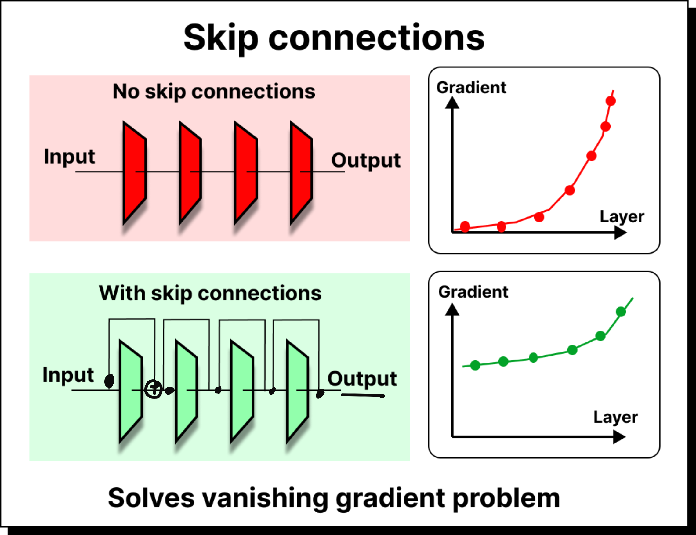
Deep networks often suffer from the vanishing gradient problem. When the loss is backpropagated to update weights, the gradient magnitude diminishes as it travels backward through many layers. This makes early layers extremely slow to learn, because their weights hardly change.
Skip connections, introduced in ResNet, solve this problem by allowing the input of a layer to bypass intermediate operations and be added directly to the output. This simple addition ensures that even if the gradient becomes small in deeper paths, there is still a strong signal flowing back through the shortcut path. Transformers adopted this idea wholeheartedly. Every sub-layer inside a transformer block has residual connections, ensuring that earlier layers remain influential and training remains stable even at great depth.
Feed-Forward Networks and Feature Enrichment
The next stage in the block is the position-wise feed-forward network. Here, each token vector is first projected into a higher dimensional space, typically four times larger than the original, and then projected back down. For example, a 768-dimensional token is expanded into 3072 dimensions, passed through a non-linear activation like ReLU or GELU, and then compressed back into 768.
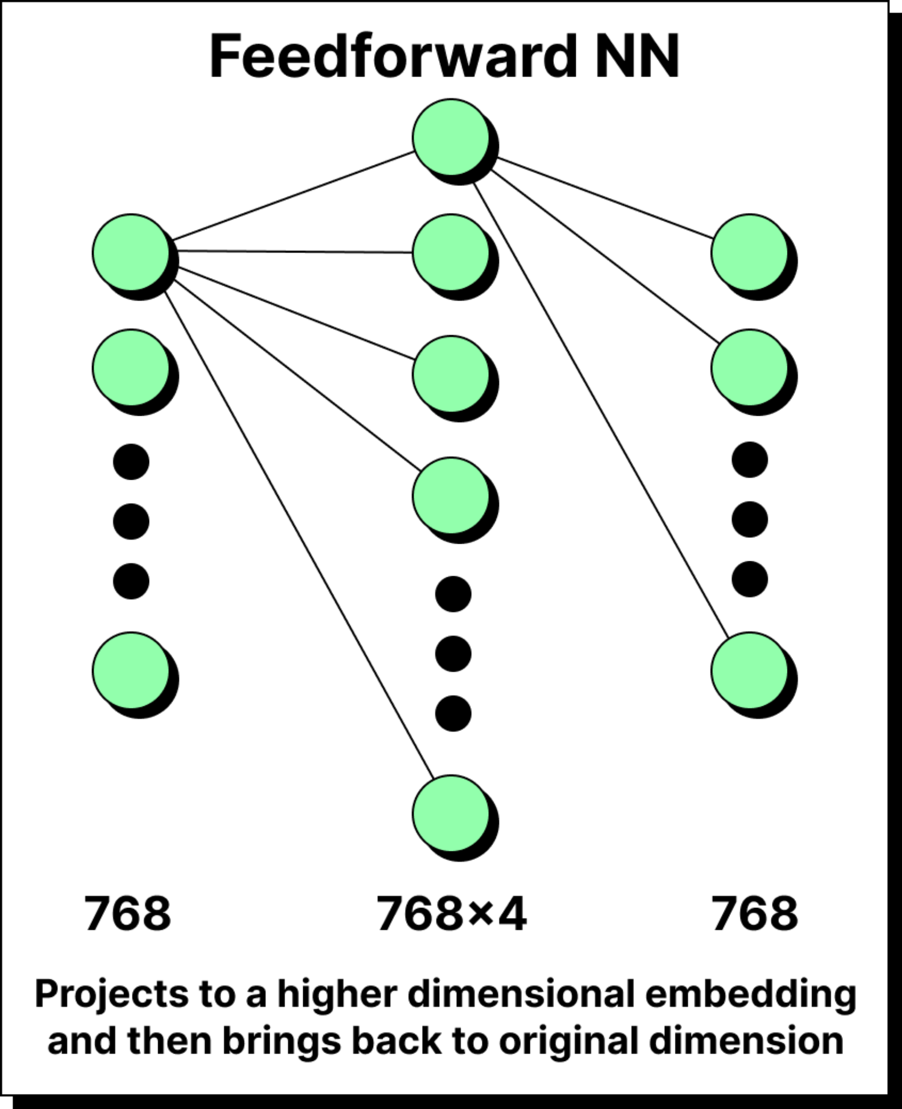
At first glance, this might seem like wasted effort. Why project up only to project back down? The reason lies in feature enrichment. Expanding into a larger space allows the model to capture richer interactions and more abstract features. If we projected downward instead, say from 768 to 300, we would lose information irreversibly. Projection upward enriches the token’s representation, projection downward prunes it back into a usable form, but the new form is more expressive than the original.
Interestingly, this feed-forward stage accounts for most of the parameters in large transformers. In GPT-3, nearly two-thirds of the 175 billion parameters are in these simple projection matrices. Multi-head attention, complex as it seems, accounts for only about one-third.
Repetition Across Blocks
The process described so far – normalization, attention, dropout, skip connections, and feed-forward projection – is repeated across many transformer blocks. In GPT-2, this sequence is repeated 12 times; in GPT-3, 96 times. Each repetition reshapes the token further, embedding it deeper into the context of the sentence. By the end, the original semantic fingerprint of cat is transformed into something almost unrecognizable – a vector that no longer just means “cat,” but “cat in the context of this sentence, after seeing all other tokens around it.”
Output Layer and Logits
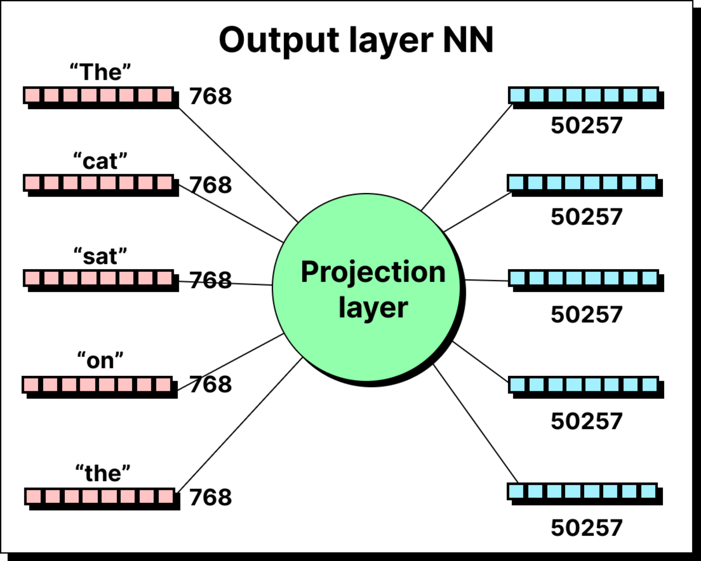
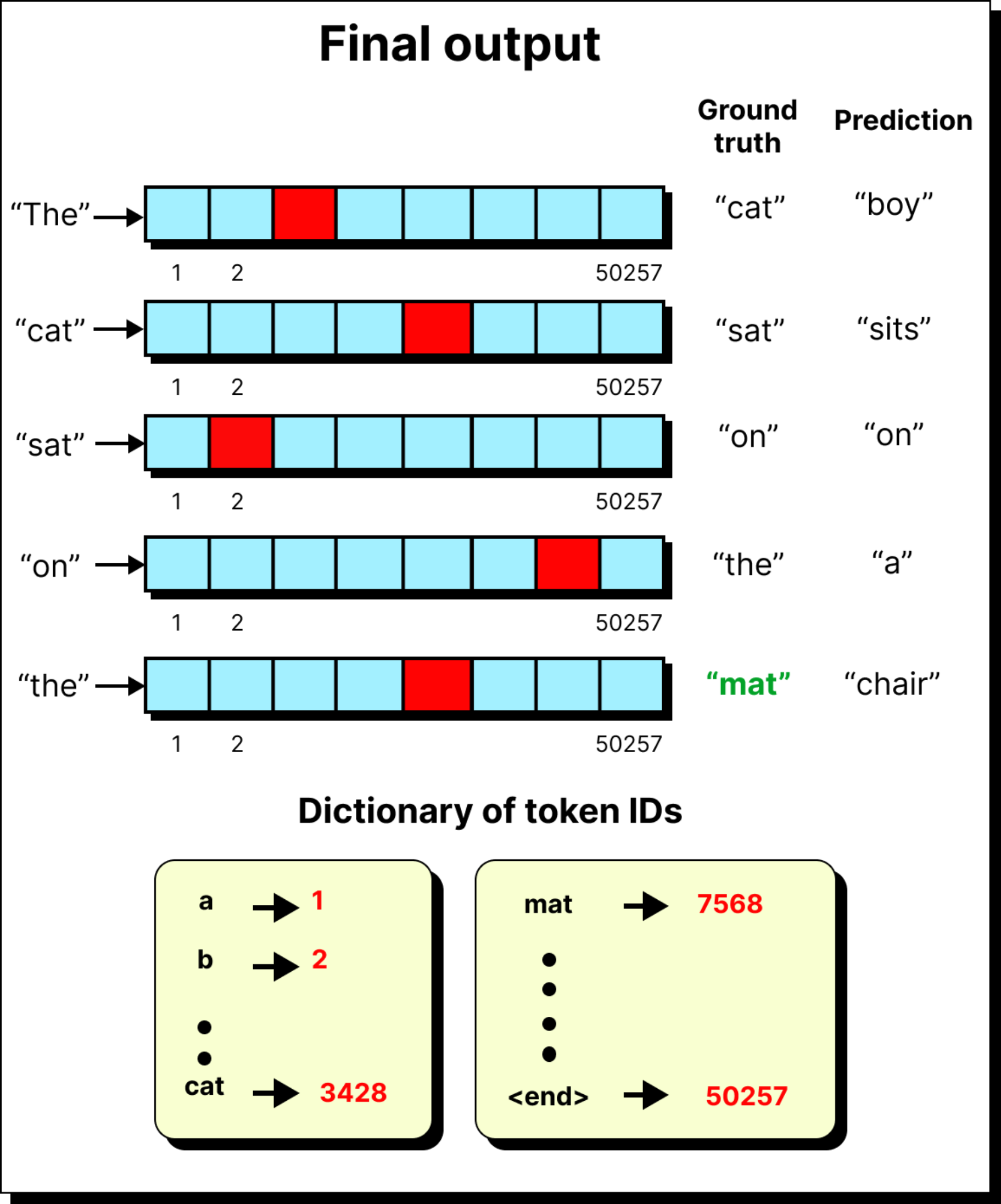
Once the token has passed through all the blocks, it reaches the output stage. The final vector is still of the hidden size, for example 768 in GPT-2. But the model’s job is next-word prediction. It must map this 768-dimensional representation into a probability distribution over the entire vocabulary, which may have fifty thousand tokens or more.
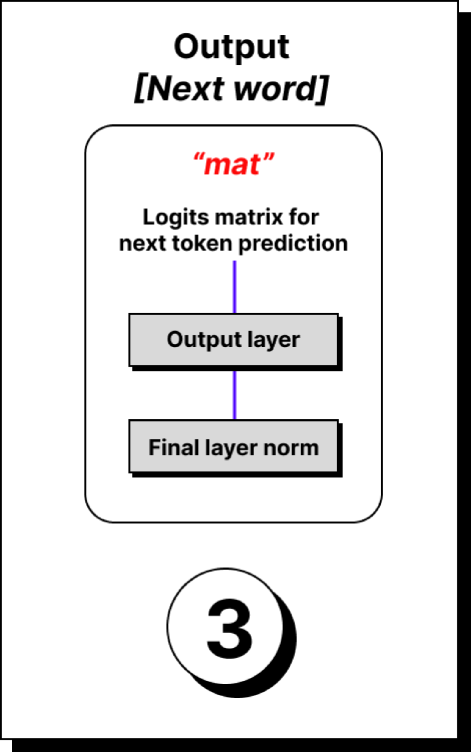
This mapping is done by multiplying the token vector with a large projection matrix of size 768 by 50,257. The result is a vector of 50,257 raw scores called logits. Each logit corresponds to one token in the vocabulary. These logits are then passed through a softmax function, which converts them into probabilities.
The highest probability token is often chosen as the next word, but sometimes sampling is applied to introduce variability. This is where parameters like temperature come in, allowing the model to occasionally pick lower probability words and appear more creative.
Looking Ahead
At this point, we have traced the entire journey of a token through the transformer – from raw input, to embeddings, to normalization, dropout, skip connections, feed-forward enrichment, and finally to the output logits and softmax probabilities.
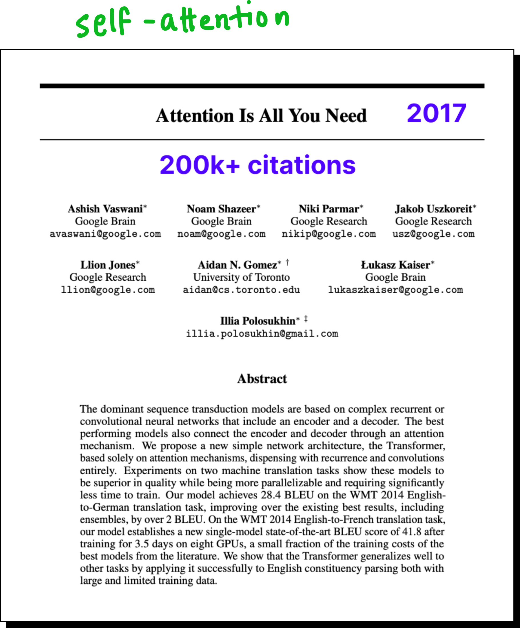
What we have not yet discussed in detail is the heart of the transformer: self-attention. That deserves its own exploration, because attention is the mechanism that allows a token to look at other tokens and gather context. In the next article, we will shift our focus to attention, starting with the original encoder-decoder models, moving to Bahdanau attention, and then finally arriving at self-attention inside transformers.
Lecture video
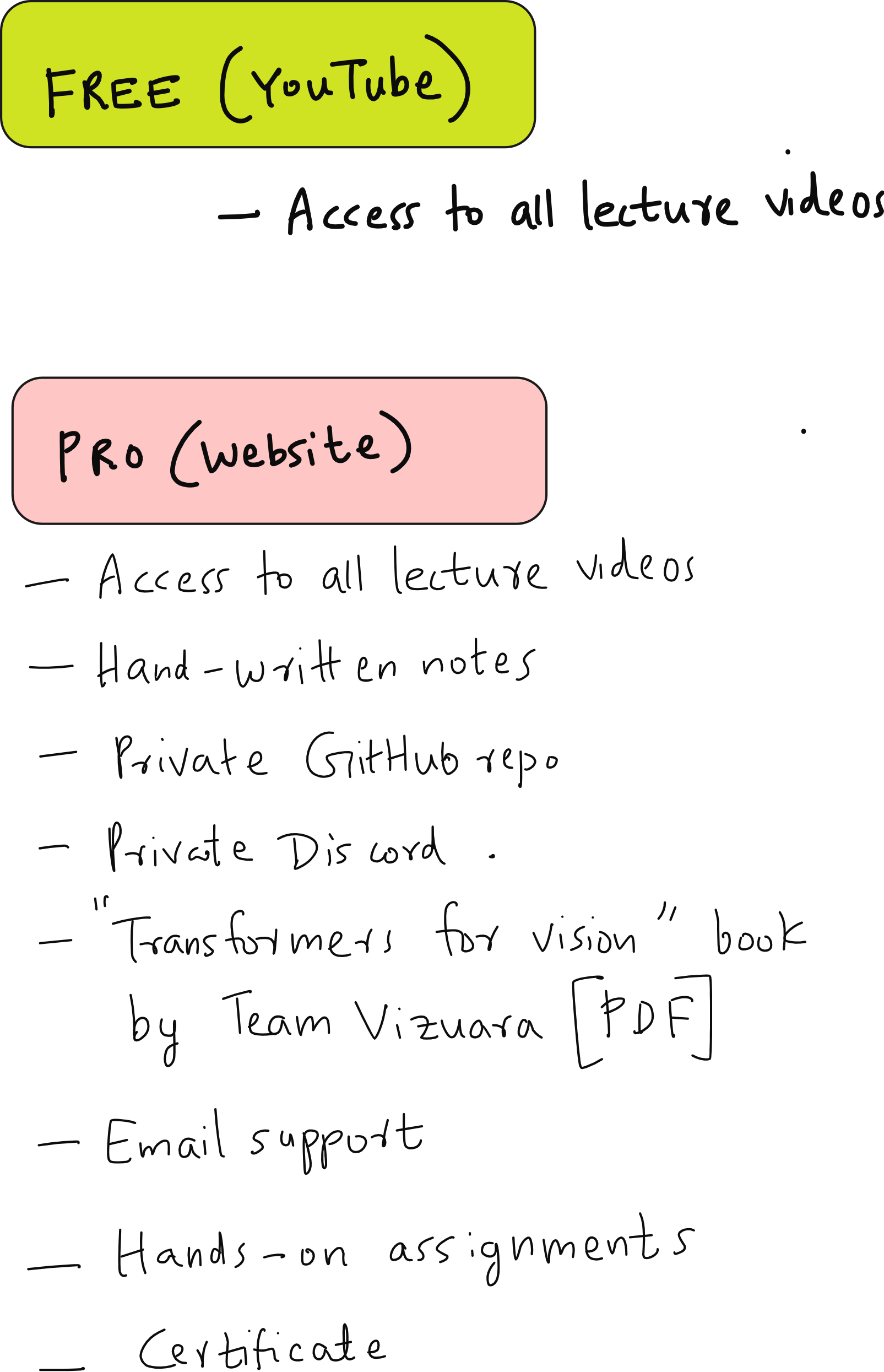
PRO content: What will you get?