Teach your neural network to "respect" Physics

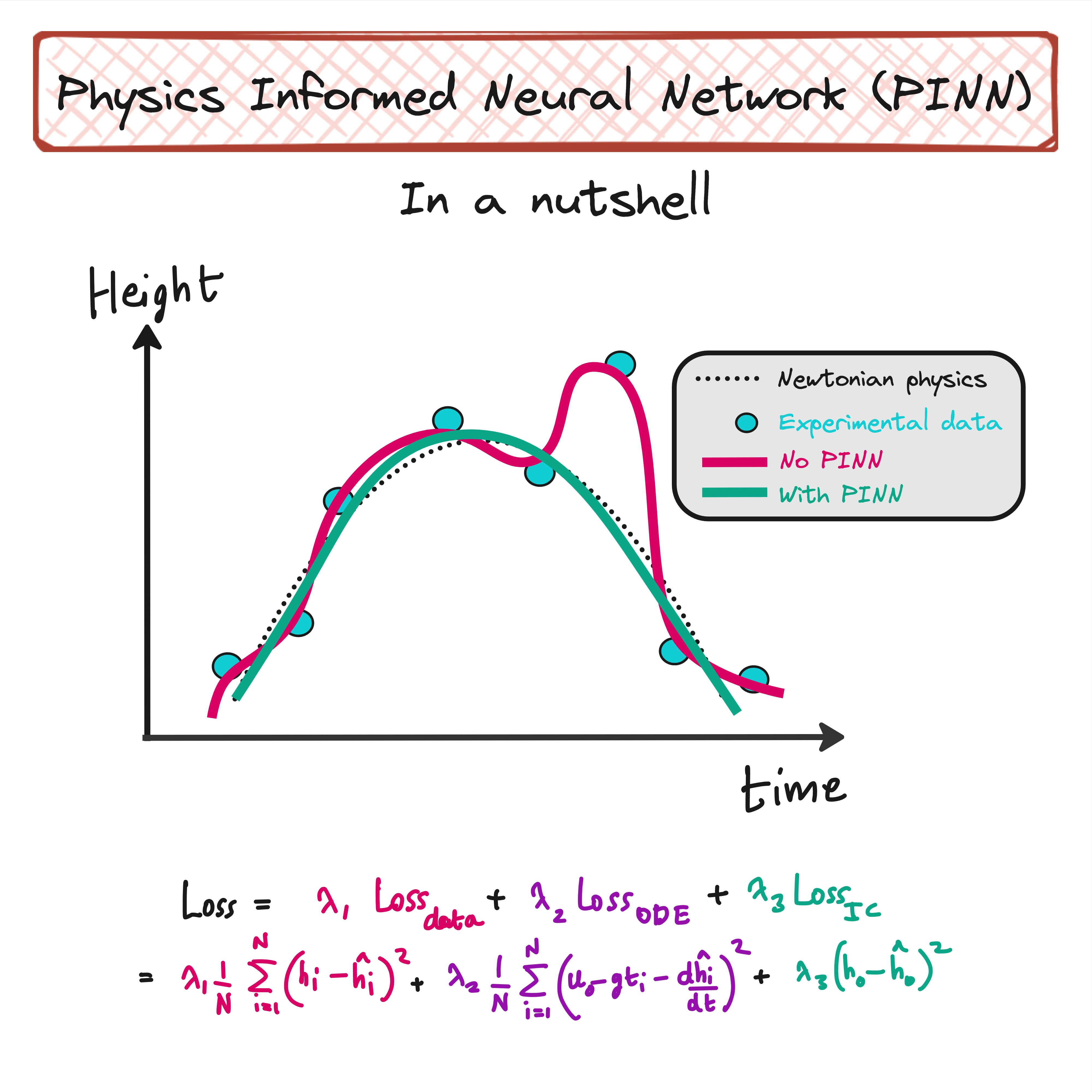
Physics Informed Neural Networks (PINN)

---

As universal function approximators, neural networks can learn to fit any dataset produced by complex functions. With deep neural networks, overfitting is not a feature. It is a bug.

Let us consider a hypothetical set of experiments. You throw a ball up (or at an angle), and note down the height of the ball at different points of time.

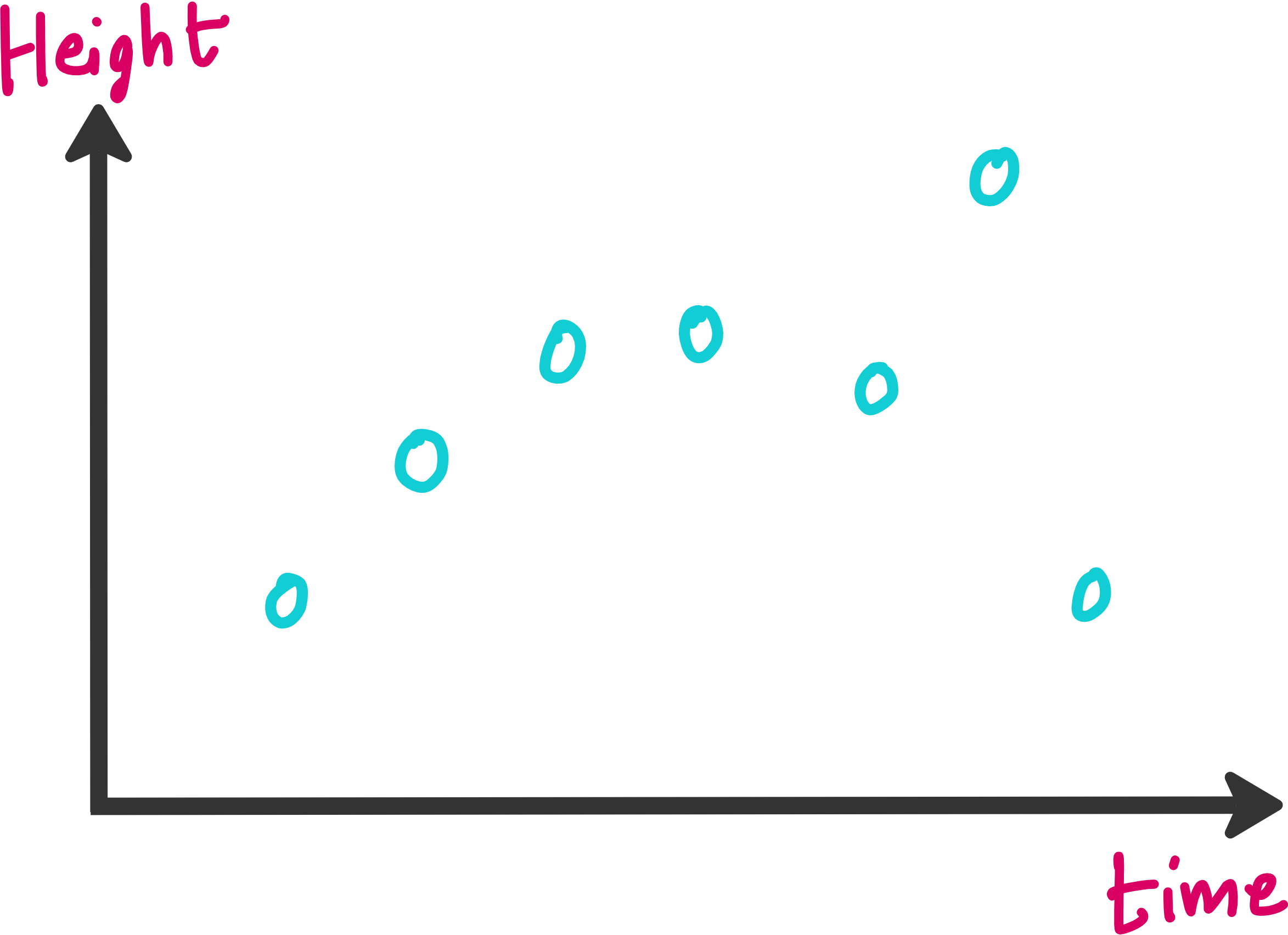
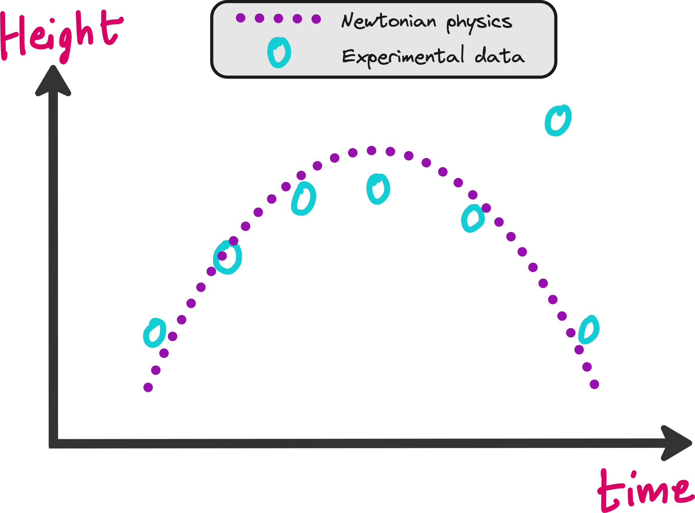
When you plot the height v/s time, you will see something like this.

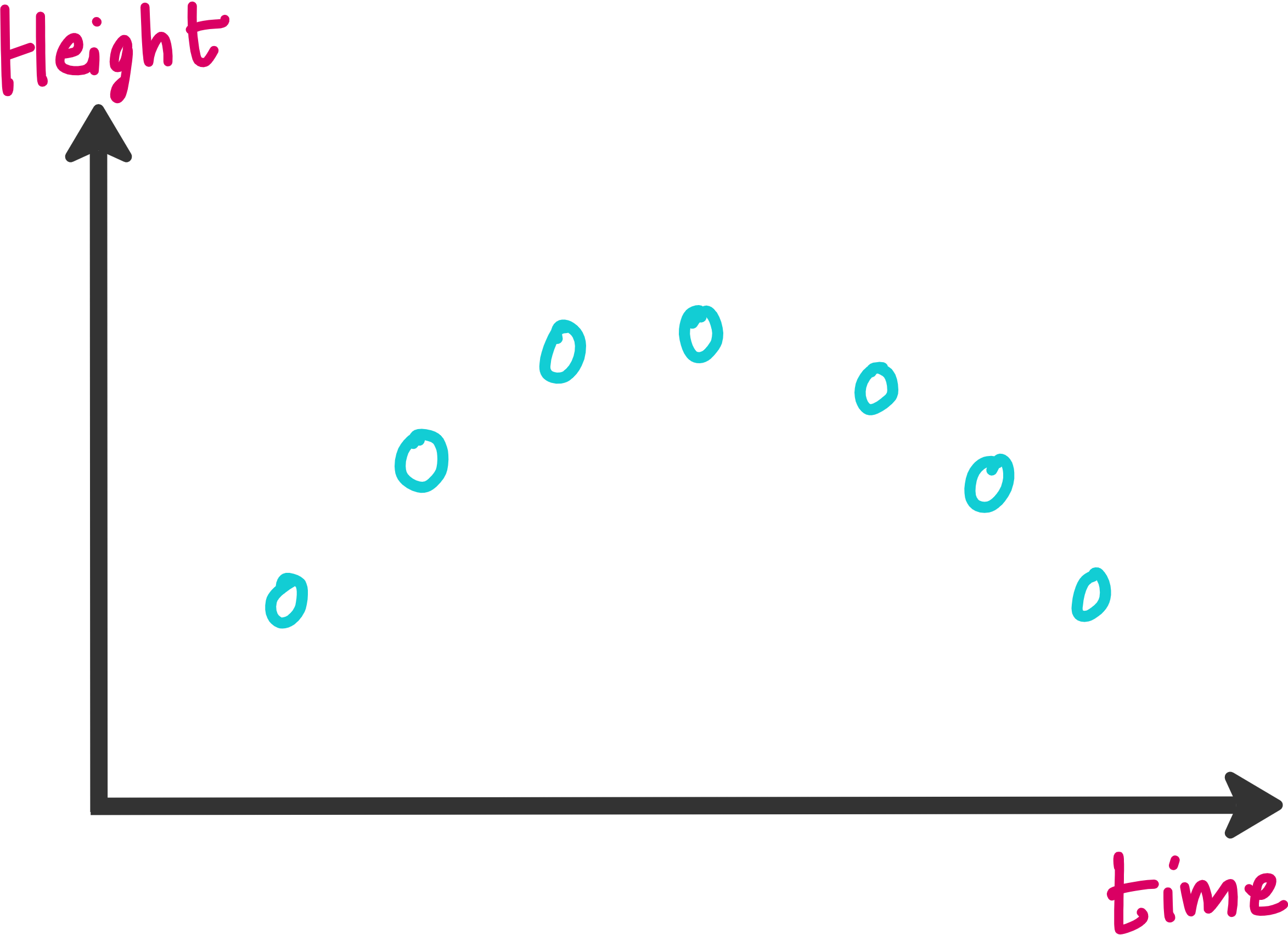
It is easy to train a neural network on this dataset so that you can predict the height of the ball even at time points where you did not note down the height in your experiments.

First let us discuss how this training is done.

Training a regular neural network

You can construct a neural network with few or multiple hidden layers. The input is time (t) and the output predicted by the neural network is height of the ball (h).

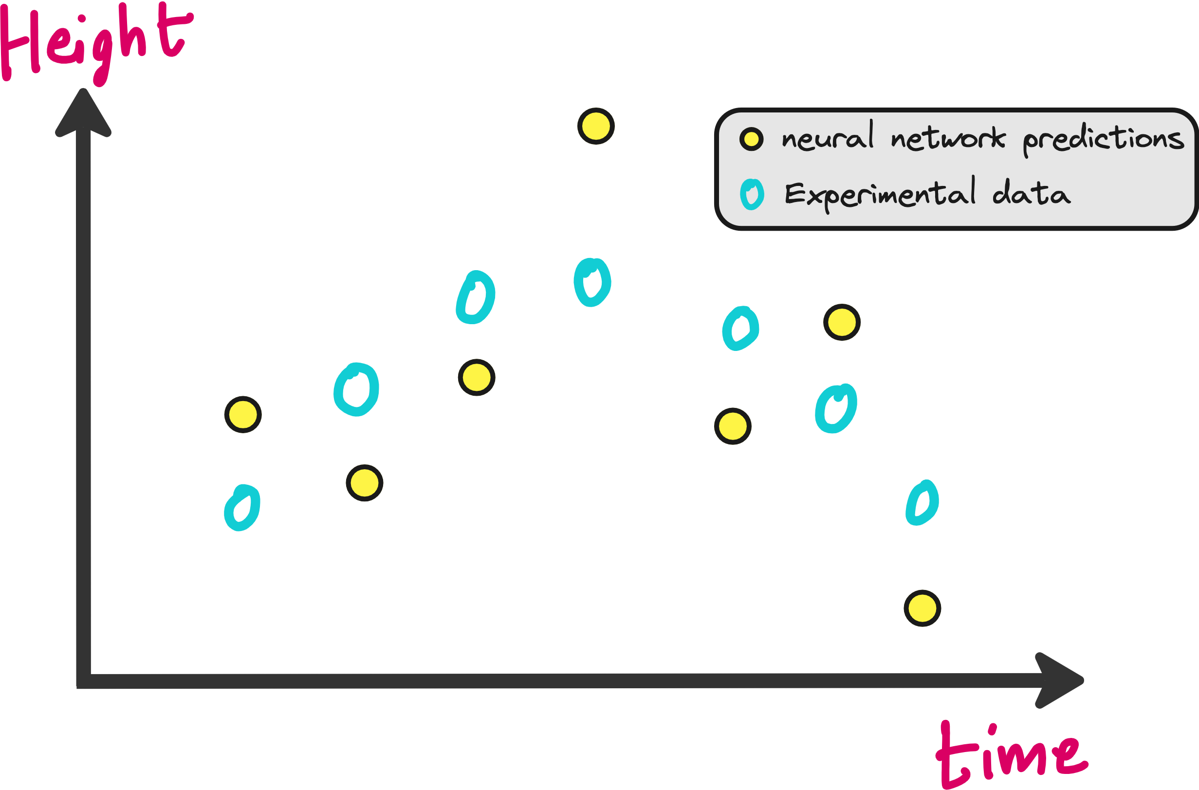
The neural network will be initialized with random weights. This means the predictions of h(t) made by the neural network will be very bad initially as shown in the image below.

We need to penalize the neural network for making these bad predictions right? How do we do that? In the form of loss functions.

Loss function

Loss of a neural network is a measure of how bad its predictions are compared the real data. The close the predictions and data, the lower the loss.

A singular goal of neural network training is to minimize the loss.

So how can we define the loss here? Consider the 3 options below.

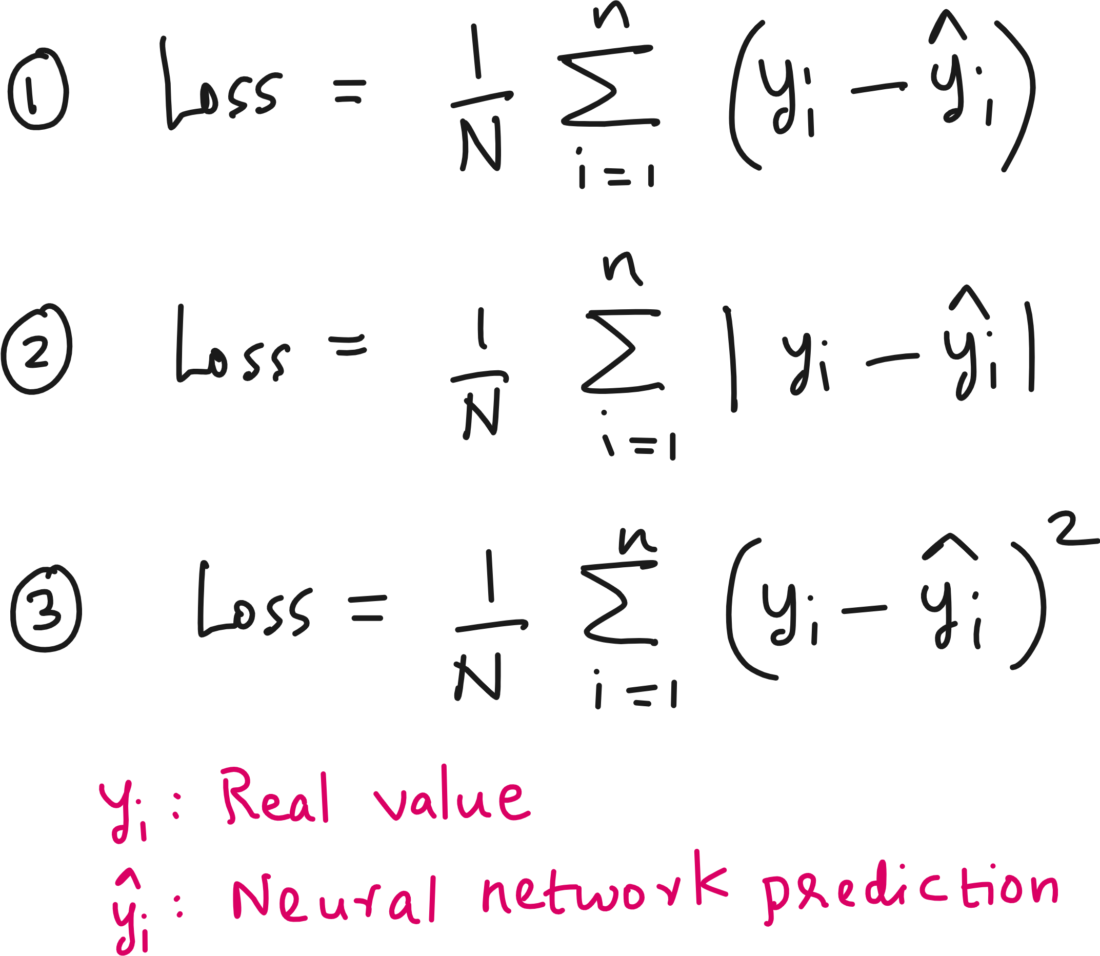
In all the 3 options, you are finding the average of some kind of loss.

• Option 1 is not good because positive and negative errors will cancel each other.

• Option 2 is okay because we are taking the absolute value of errors, but the problem is modulus function is not differentiable at x=0.

• Option 3 is the best. It is a square function which means individual errors are converted to positive numbers and the function is differentiable. This is the famous Mean Squared Error (MSE). You are taking the mean value of the square of all individual errors.

Here error means the difference between actual value and predicted value.

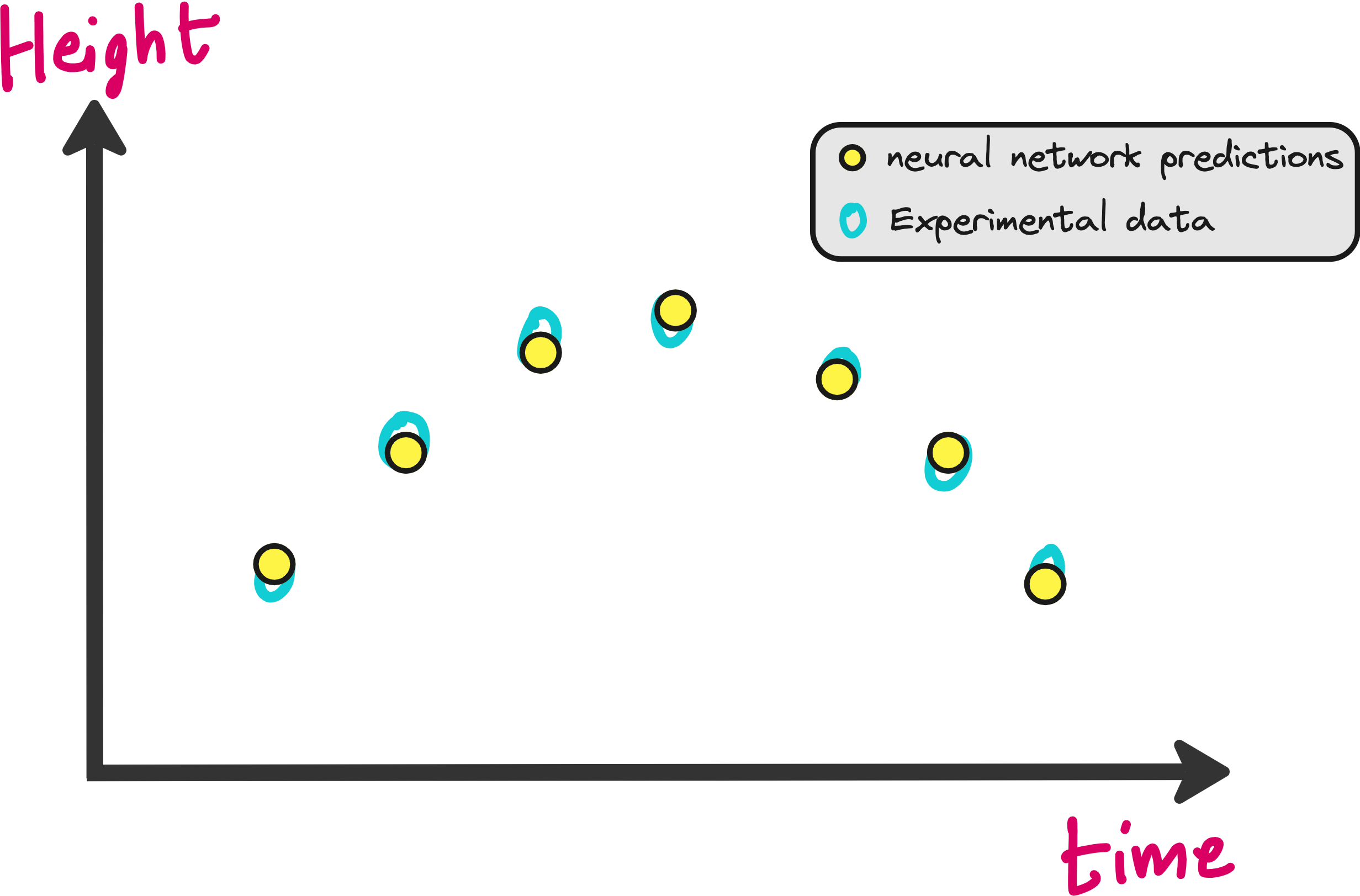
Mean Squared Error is minimum when the predictions are very close to the experimental data as shown in the figure below.

But there is a problem with this approach. What if your experimental data was not good? In the image below you can see that one of the data points is not following the trend shown by the rest of the dataset.

There can be multiple reasons due to which such data points show up in the data.

1. You did not perform the experiments well. You made a manual mistake while noting the height.

2. The sensor or instrument using which you were making the height measurement was faulty.

3. A sudden gush of wind caused a sudden jump in the height of the ball.

There could be many possibilities that results in outliers and noise in a dataset.

Knowing that real life data may have noise and outliers, it will not be wise if we train a neural network to exactly mimic this dataset. It results in something called as overfitting.

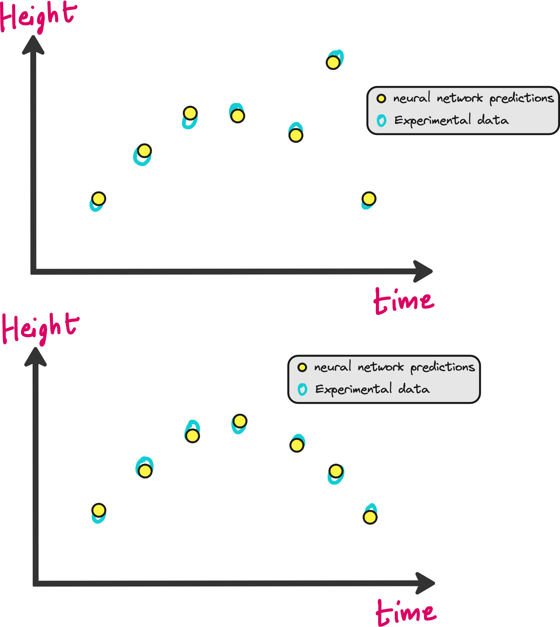
In the figure above, mean squared error will be low in both cases. However in one case neural network is fitting on outlier also, which is not good. So what should we do?

Bring physics into the picture

If you are throwing a ball and observing its physics, then you already have some knowledge about the trajectory of the ball, based on Newton’s laws of motion.

Sure, you may be making simplifications by assuming that the effect of wind or air drag or buoyancy are negligible. But that does not take away from the fact that you already have decent knowledge about this system even in the absence of a trained neural network.

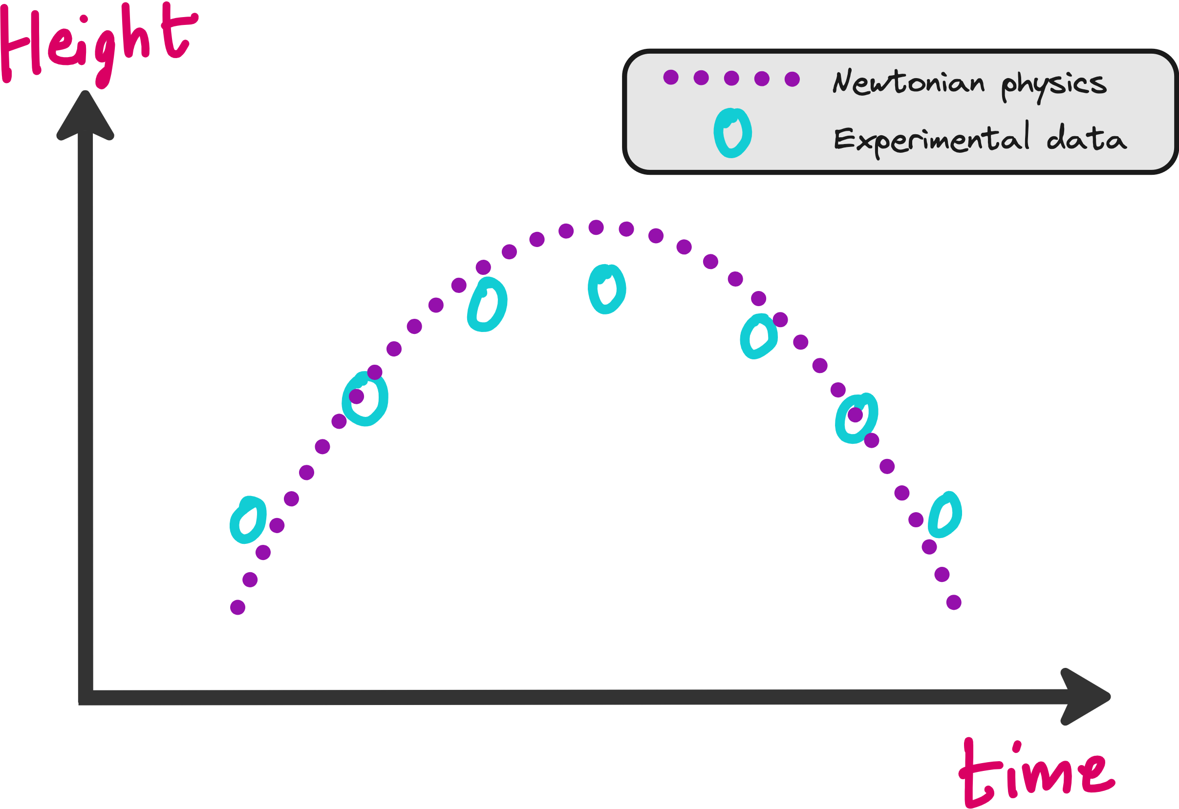
The physics you assume may not be in perfect agreement with the experimental data as shown above, but it makes sense to think that the experiments will not deviate too much from physics.

So if one of your experimental data points deviate too much from what physics says, there is probably something wrong with that data point. So how can you let you neural network take care of this?

How can you teach physics to neural networks?

If you want to teach physics to neural network, then you have to somehow incentivize neural network to make predictions closer to what is suggested by physics.

If the neural network makes a prediction where the height of the ball is far away from the purple dotted line, then loss should increase.

If the predictions are closer to the dotted line, then the loss should be minimum.

What does this mean? Modify the loss function.

How can you modify the loss function such that the loss is high when predictions deviate from physics? And how does this enable the neural network make more physically sensible predictions? Enter PINN - Physics Informed Neural Network.

Physics Informed Neural Network (PINN)

The goal of PINNs is to solve (or learn solutions to) differential equations by embedding the known physics (or governing differential equations) directly into the neural network’s training objective (loss function).

The idea of PINNs were introduced in this seminal paper by Maziar Raissi et. al.: https://maziarraissi.github.io/PINNs/

The basic idea in PINN is to have a neural network is trained to minimize a loss function that includes:

1. A data mismatch term (if observational data are available).

2. A physics loss term enforcing the differential equation itself (and initial/boundary conditions).

Let us implement PINN on our example

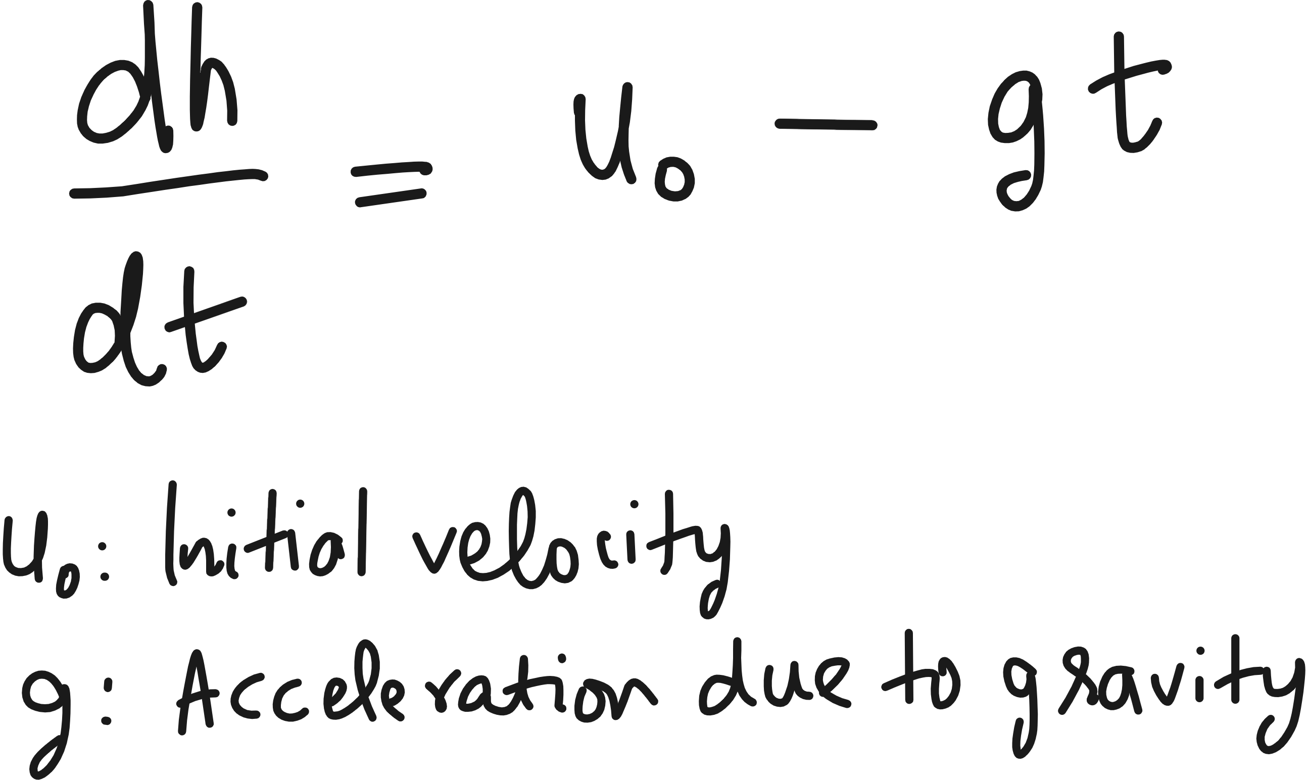
Let us look at what we know about our example. When a ball is thrown up, it trajectory h(t) varies according to the following ordinary differential equation (ODE).

However this ODE alone cannot fully describe h(t) uniquely. You also need an initial condition. Mathematically this is because to solve a first-order differential equation in time, you need 1 initial condition.

Logically, to know height as a function of time, you need to know the starting height from which the ball was thrown. Look at the image below. In both cases, the balls are thrown at the exact same time with the exact same initial velocity component in the vertical direction. But the h(t) depends on the initial height. So you need to know h(t=0) for fully describing the height of the ball as a function of time.

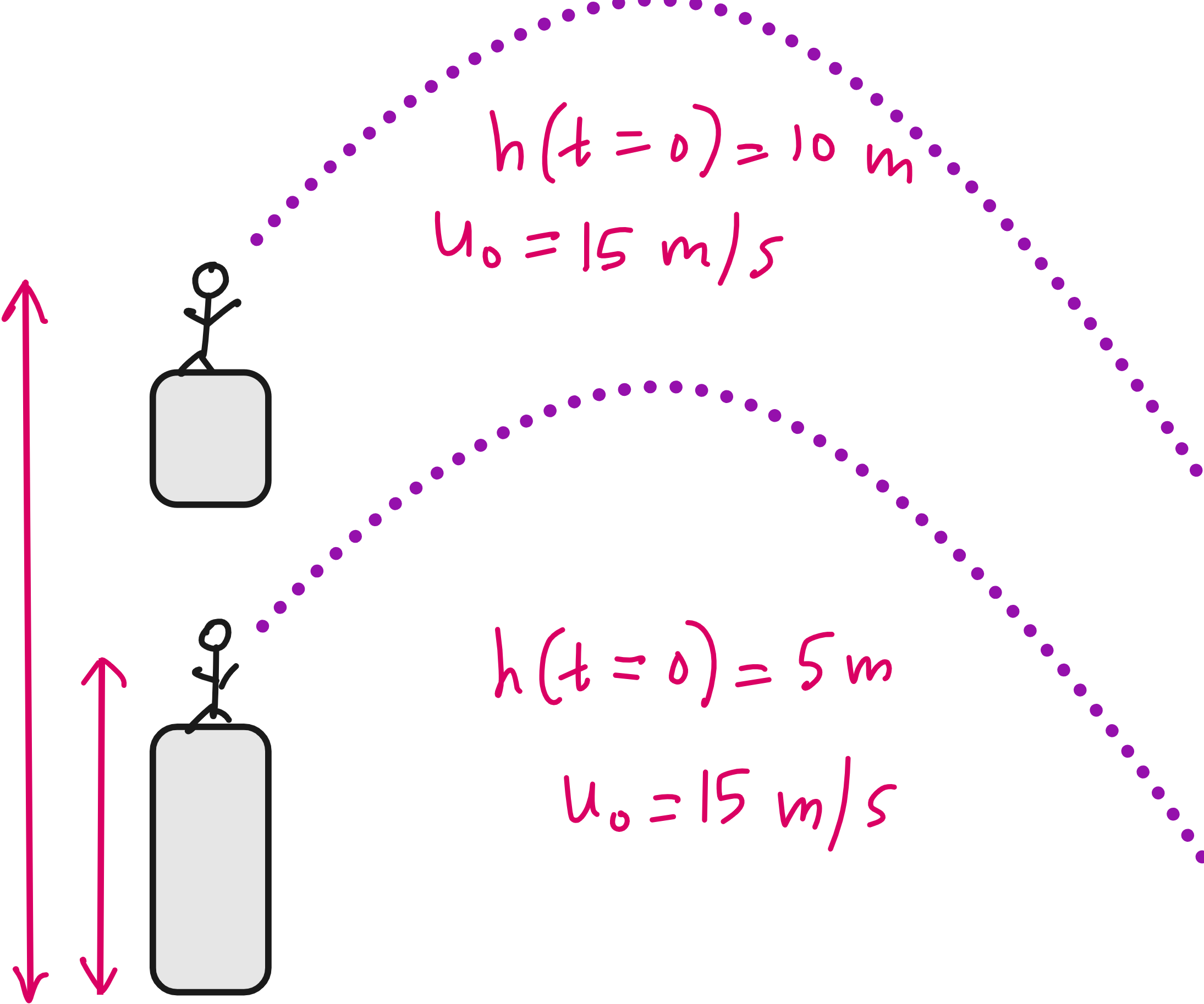
This means it is not enough to make the neural network make accurate predictions on dh/dt, the neural network should also make accurate prediction on h(t=0) for fully matching the physics in this case.

Loss due to dh/dt (ODE loss)

We know the expected dh/dt because we know the initial velocity and acceleration due to gravity.

How do we get the dh/dt predicted by the neural network? After all it is predicting height h, not velocity v or dh/dt. The answer is Automatic differentiation (AD).

Because most machine‐learning frameworks (e.g., TensorFlow, PyTorch, JAX) support automatic differentiation, you can compute dh/dt by differentiating the neural network.

Thus, we have a predicted dh/dt (from the neural network differentiation) for every experimental time points, and we have an actual dh/dt based on the physics.

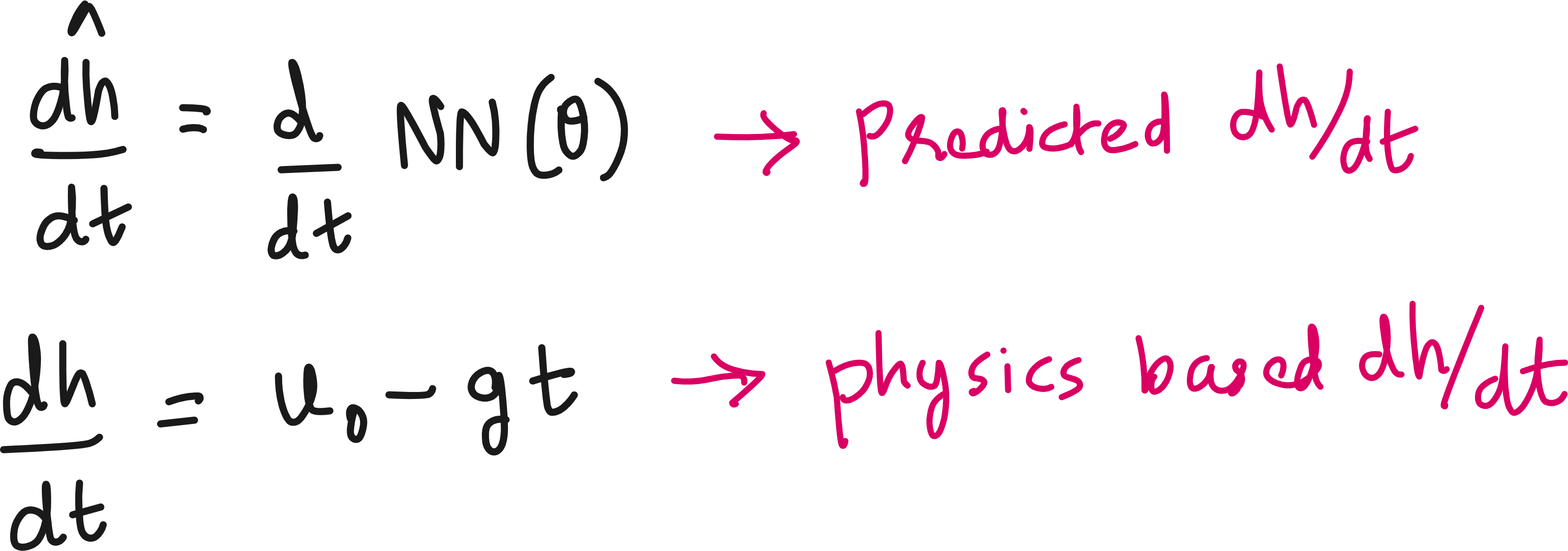
Now we can define a loss due to the difference between predicted and physics-based dh/dt.

Minimizing this loss (which I prefer to call ODE loss) is a good thing to ensure that neural network learns the ODE. But that is not enough. We need to make the neural network follow the initial condition also. That brings us to the next loss term.

Initial condition loss

This is easy. You know the initial condition. You make the neural network make a prediction of height for t=0. See how far off the prediction is from the reality. You can construct a squared error which can be called as the Initial Condition Loss.

So is that it? You have ODE loss and Initial condition loss. Is it enough that the neural network tries to minimize these 2 losses? What about the experimental data? There are 3 things to consider.

1. You cannot throw away the experimental data.

2. You cannot neglect the physics described by the ODEs or PDEs.

3. You cannot neglect the initial and/or boundary conditions.

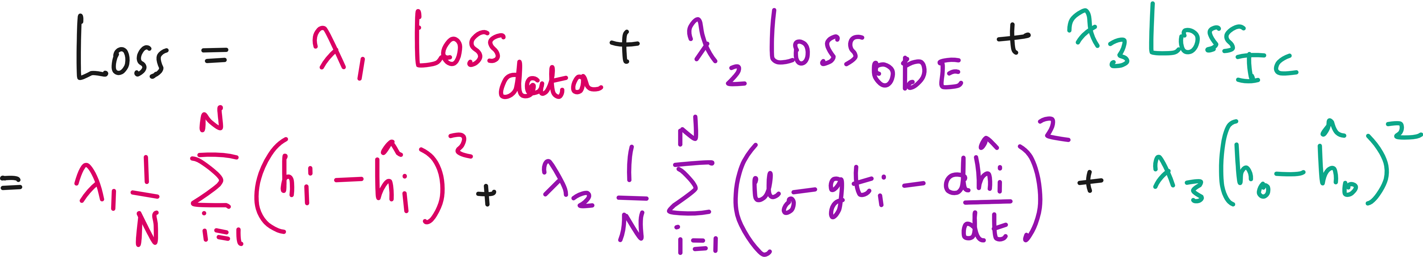
Thus you have to also consider the data-based mean squared error loss along with ODE loss and Initial condition loss.

The modified loss term

The simple mean squared error based loss term can now be modified like below.

If there are boundary conditions in addition to initial conditions, you can add an additional term based on the difference between predicted boundary conditions and actual boundary conditions.

Here the Data loss term ensures that the predictions are not too far from the experimental data points.

The ODE loss term + the initial condition loss term ensures that the predictions are not too far from what described by the physics.

If you are pretty sure about the physics the you can set λ1 to zero. In the ball throwing experiment, you will be sure about the physics described by our ODE if air drag, wind, buoyancy and any other factors are ignored. Only gravity is present. And in such cases, the PINN effectively becomes an ODE solver.

However, for real life cases where only part of the physics is known or if you are not fully sure of the ODE, then you retain λ1 and other λ terms in the net loss term. That way you force the neural network to respect physics as well as the experimental data. This also suppress the effects of experimental noise and outliers.

In short, in Physics Informed Neural Networks (PINN), you are “informing” the neural network that some physics is there behind the data in the form of modified loss function. It is a simple and fascinating concept.

Lecture video

I have made a 60 minute lecture video on PINNs (meant even for absolute beginners) and hosted it on Vizuara’s YouTube channel. Do check this out. I hope you enjoy watching this lecture as much as I enjoyed making it.

Python implementation

Import required libraries

import torch
import torch.nn as nn
import numpy as np
import matplotlib.pyplot as plt

Generate Synthetic Data

# --------------------------
# 1. Generate Synthetic Data
# --------------------------

# Physics parameters
g = 9.8        # acceleration due to gravity
h0 = 1.0       # initial height
v0 = 10.0      # initial velocity

# True (analytical) solution h(t) = h0 + v0*t - 0.5*g*t^2
def true_solution(t):
    return h0 + v0*t - 0.5*g*(t**2)

# Generate some time points
t_min, t_max = 0.0, 2.0
N_data = 10
t_data = np.linspace(t_min, t_max, N_data)

# Generate synthetic "experimental" heights with noise
np.random.seed(0)
noise_level = 0.7
h_data_exact = true_solution(t_data)
h_data_noisy = h_data_exact + noise_level*np.random.randn(N_data)

# Convert to PyTorch tensors
t_data_tensor = torch.tensor(t_data, dtype=torch.float32).view(-1, 1)
h_data_tensor = torch.tensor(h_data_noisy, dtype=torch.float32).view(-1, 1)

Define a small feed-forward neural network for h(t)

# --------------------------------------------------------
# 2. Define a small feed-forward neural network for h(t)
# --------------------------------------------------------
class PINN(nn.Module):
    def __init__(self, n_hidden=20):
        super(PINN, self).__init__()
        # A simple MLP with 2 hidden layers
        self.net = nn.Sequential(
            nn.Linear(1, n_hidden),
            nn.Tanh(),
            nn.Linear(n_hidden, n_hidden),
            nn.Tanh(),
            nn.Linear(n_hidden, 1)
        )

    def forward(self, t):
        """
        Forward pass: input shape (batch_size, 1) -> output shape (batch_size, 1)
        """
        return self.net(t)

# Instantiate the model
model = PINN(n_hidden=20)

Helper for Automatic Differentiation

# --------------------------------
# 3. Helper for Automatic Diff
# --------------------------------
def derivative(y, x):
    """
    Computes dy/dx using PyTorch's autograd.
    y and x must be tensors with requires_grad=True for x.
    """
    return torch.autograd.grad(
        y, x,
        grad_outputs=torch.ones_like(y),
        create_graph=True
    )[0]

Define the Loss Components (PINN)

# ----------------------------------------
# 4. Define the Loss Components (PINN)
# ----------------------------------------

# We have:
#    (1) Data loss (fit noisy data)
#    (2) ODE loss: dh/dt = v0 - g * t
#    (3) Initial condition loss: h(0) = h0

def physics_loss(model, t):
    """
    Compare d(h_pred)/dt with the known expression (v0 - g t).
    """
    # t must have requires_grad = True for autograd to work
    t.requires_grad_(True)

    h_pred = model(t)
    dh_dt_pred = derivative(h_pred, t)

    # For each t, physics says dh/dt = v0 - g * t
    dh_dt_true = v0 - g * t

    loss_ode = torch.mean((dh_dt_pred - dh_dt_true)**2)
    return loss_ode

def initial_condition_loss(model):
    """
    Enforce h(0) = h0.
    """
    # Evaluate at t=0
    t0 = torch.zeros(1, 1, dtype=torch.float32, requires_grad=False)
    h0_pred = model(t0)
    return (h0_pred - h0).pow(2).mean()

def data_loss(model, t_data, h_data):
    """
    MSE between predicted h(t_i) and noisy measurements h_data.
    """
    h_pred = model(t_data)
    return torch.mean((h_pred - h_data)**2)

Training Setup

# ---------------------------------------
# 5. Training Setup
# ---------------------------------------
optimizer = torch.optim.Adam(model.parameters(), lr=0.01)

# Hyperparameters for weighting the loss terms
lambda_data = 2.0
lambda_ode  = 2.0
lambda_ic   = 2.0

# For logging
num_epochs = 4000
print_every = 200

Training Loop

# ---------------------------------------
# 6. Training Loop
# ---------------------------------------
model.train()
for epoch in range(num_epochs):
    optimizer.zero_grad()

    # Compute losses
    l_data = data_loss(model, t_data_tensor, h_data_tensor)
    l_ode  = physics_loss(model, t_data_tensor)
    l_ic   = initial_condition_loss(model)

    # Combined loss
    loss = lambda_data * l_data + lambda_ode * l_ode + lambda_ic * l_ic

    # Backprop
    loss.backward()
    optimizer.step()

    # Print progress
    if (epoch+1) % print_every == 0:
        print(f"Epoch {epoch+1}/{num_epochs}, "
              f"Total Loss = {loss.item():.6f}, "
              f"Data Loss = {l_data.item():.6f}, "
              f"ODE Loss = {l_ode.item():.6f}, "
              f"IC Loss = {l_ic.item():.6f}")

Evaluate the Trained Model

# ---------------------------------------
# 7. Evaluate the Trained Model
# ---------------------------------------
model.eval()
t_plot = np.linspace(t_min, t_max, 100).reshape(-1, 1).astype(np.float32)
t_plot_tensor = torch.tensor(t_plot, requires_grad=True)
h_pred_plot = model(t_plot_tensor).detach().numpy()

# True solution (for comparison)
h_true_plot = true_solution(t_plot)

# Plot results
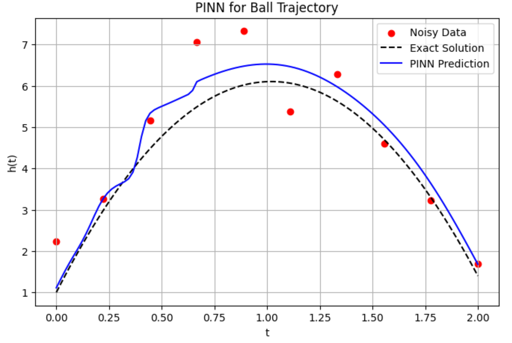
plt.figure(figsize=(8, 5))
plt.scatter(t_data, h_data_noisy, color='red', label='Noisy Data')
plt.plot(t_plot, h_true_plot, 'k--', label='Exact Solution')
plt.plot(t_plot, h_pred_plot, 'b', label='PINN Prediction')
plt.xlabel('t')
plt.ylabel('h(t)')
plt.legend()
plt.title('PINN for Ball Trajectory')
plt.grid(True)
plt.show()