
RMSprop Gradient Descent from Scratch
With a recap of vanilla/normal/batch gradient descent


Optimization in machine learning is all about finding that sweet spot—a set of parameters that minimizes error. While Gradient Descent laid the foundation for this, its practical limitations called several upgrades. In this article we will discuss RMSprop (root mean square propagation) where you can adjust the learning rate based on the history of past gradients. We will also implement RMSprop from scratch.

Recap of Gradient Descent and Its Shortcomings
What Is Gradient Descent?
Gradient Descent is an iterative optimization algorithm used to minimize a loss function L(θ). At each step, it updates the model parameters θ by moving in the direction opposite to the gradient of the loss function with respect to θ:
Here:
∇L(θ): Gradient of the loss function.
η: Learning rate (step size).
Key Properties:
It computes the gradient over the entire dataset at each step.
Guarantees a smooth and steady descent towards the minimum of L(θ)
The Struggles of Vanilla Gradient Descent
Computational Overhead: Calculating the gradient over the entire dataset is computationally expensive for large datasets.
Example: For a dataset with N samples, computing the gradient requires N operations per update.
Slow Convergence: Gradient Descent can take small, steady steps and struggle with large datasets or complex loss landscapes.
Local Minima or Saddle Points: It may get stuck in a local minimum or wander in a flat saddle region, delaying convergence.
These limitations led to the development of Stochastic Gradient Descent, which makes optimization faster and more flexible.
NOTE: The “normal” gradient descent is also called as vanilla gradient descent or batch gradient descent (BGD). Batch because the parameter update is calculated with respect to all data points in the batch.
RMSprop: A Smarter Way to Tame Learning Rates (η) in Machine Learning
Training machine learning models often feels like balancing on a tightrope. Use a learning rate that’s too high, and your optimization jumps around without ever converging. Use one that’s too low, and progress crawls. RMSprop is an optimization algorithm designed to address this delicate balancing act by adapting learning rates dynamically for each parameter.
RMSprop, short for Root Mean Square Propagation, is an optimization algorithm that adapts the learning rate for each parameter by scaling it inversely with the square root of the parameter’s gradient history. The algorithm was proposed by Geoffrey Hinton in one of his online lectures and quickly became a favorite for training deep neural networks.
How RMSprop Works
RMSprop achieves its adaptive learning rates by maintaining a moving average of the squared gradients for each parameter. The key steps are:
Compute the Gradient: Calculate the gradient of the loss function with respect to each parameter.
Update the Running Average: Smooth the squared gradients using an exponentially decaying average:
\(G_t = \beta G_{t-1} + (1 - \beta) (\nabla \theta)^2 \)Here:
Gt: The running average of squared gradients at time t.
β: The decay rate (commonly 0.9).
Scale the learning rate: Divide the learning rate by the square root of the running average, plus a small constant ϵ to prevent division by zero:
\(\text{Learning rate} = \frac{\eta}{\sqrt{G_t} + \epsilon} \)
Update Parameters: Use the scaled gradient to update parameters:
Where η is the learning rate
Why RMSprop Works
1. Adaptive Learning Rates
RMSprop’s use of squared gradient averages ensures that parameters with large gradients get smaller updates, while those with small gradients receive larger updates. This adaptability allows RMSprop to efficiently traverse complex optimization landscapes.
2. Handles Exploding and Vanishing Gradients
By normalizing the gradients, RMSprop prevents excessive updates caused by large gradients, and boosts updates in regions with tiny gradients. This is especially useful in deep networks, where gradients often explode or vanish as they propagate backward through the layers.
3. Faster Convergence
In regions where the optimization path is steep or flat, RMSprop adjusts the learning rates dynamically, accelerating convergence compared to standard Gradient Descent.
Advantages of SGD
Speed: Faster updates as only a single data point is used, making it ideal for large datasets.
Escaping Local Minima: The noise introduced by random updates helps SGD escape local minima and explore the parameter space.
Scalability: Works well for streaming data or online learning, where data arrives in small batches.
Code implementation of RMSprop v/s Vanilla Gradient Descent
import numpy as np
import matplotlib.pyplot as plt
def quadratic_loss(x, y):
return x**2 + 10 * y**2
def quadratic_grad(x, y):
dx = 2 * x
dy = 20 * y
return np.array([dx, dy])
def gradient_descent(grad_func, lr, epochs, start_point):
x, y = start_point
path = [(x, y)]
losses = [quadratic_loss(x, y)]
for _ in range(epochs):
grad = grad_func(x, y)
x -= lr * grad[0]
y -= lr * grad[1]
path.append((x, y))
losses.append(quadratic_loss(x, y))
return np.array(path), losses
def rmsprop_optimizer(grad_func, lr, beta, epsilon, epochs, start_point):
x, y = start_point
Eg2 = np.array([0.0, 0.0]) # Moving average of squared gradients
path = [(x, y)]
losses = [quadratic_loss(x, y)]
for _ in range(epochs):
grad = grad_func(x, y) # Compute gradients
Eg2 = beta * Eg2 + (1 - beta) * (grad ** 2) # Update moving average
x -= lr * grad[0] / (np.sqrt(Eg2[0]) + epsilon) # Update x
y -= lr * grad[1] / (np.sqrt(Eg2[1]) + epsilon) # Update y
path.append((x, y))
losses.append(quadratic_loss(x, y))
return np.array(path), losses
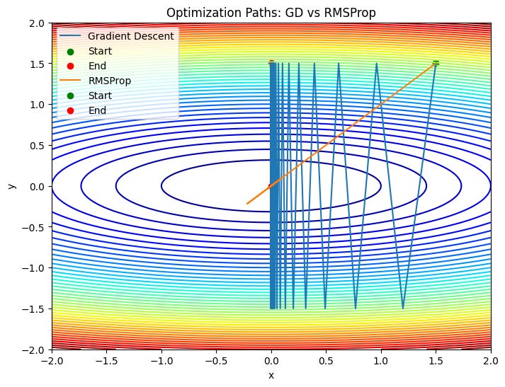
def plot_paths(function, paths, labels, title):
X, Y = np.meshgrid(np.linspace(-2, 2, 400), np.linspace(-2, 2, 400))
Z = function(X, Y)
plt.figure(figsize=(8, 6))
plt.contour(X, Y, Z, levels=50, cmap='jet')
for path, label in zip(paths, labels):
plt.plot(path[:, 0], path[:, 1], label=label)
plt.scatter(path[0, 0], path[0, 1], color='green', label="Start")
plt.scatter(path[-1, 0], path[-1, 1], color='red', label="End")
plt.title(title)
plt.xlabel("x")
plt.ylabel("y")
plt.legend()
plt.show()
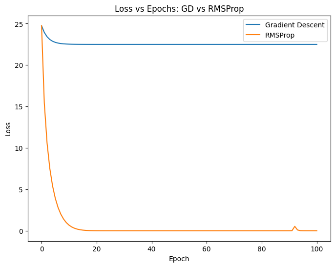
def plot_losses(losses, labels, title):
plt.figure(figsize=(8, 6))
for loss, label in zip(losses, labels):
plt.plot(loss, label=label)
plt.title(title)
plt.xlabel("Epoch")
plt.ylabel("Loss")
plt.legend()
plt.show()
lr_gd = 0.1 # Learning rate for GD
lr_rmsprop = 0.1 # Learning rate for RMSProp
beta = 0.9 # Decay rate for RMSProp
epsilon = 1e-8 # Small constant for RMSProp
epochs = 100
start_point = (1.5, 1.5) # Initial point far from the minimum
path_gd, losses_gd = gradient_descent(quadratic_grad, lr_gd, epochs, start_point)
path_rmsprop, losses_rmsprop = rmsprop_optimizer(quadratic_grad, lr_rmsprop, beta, epsilon, epochs, start_point)
plot_paths(quadratic_loss, [path_gd, path_rmsprop],
["Gradient Descent", "RMSProp"],
"Optimization Paths: GD vs RMSProp")
plot_losses([losses_gd, losses_rmsprop],
["Gradient Descent", "RMSProp"],
"Loss vs Epochs: GD vs RMSProp")