Recover unknown "science" using Machine Learning

How Universal Differential Equations are replacing traditional black-box models

Neural Networks, as you know, are called as “blackbox” because although they can train to fit through any data, you don’t know what is going on inside. Neural Networks are therefore capable to make predictions that violate basic physics or even laws of thermodynamics.

To fix this issue, Machine Learning scientists introduced PINNs - Physics Informed Neural Networks - where you penalize a neural network when it makes physically non-sense predictions.

But what if you don’t know the full physics of a system? How do you penalized the neural network in that case?

Universal Differential Equations (UDE) is the answer.

I am writing this article in praise of this marvelous technique that is truly changing the way we are looking at how to bring science and ML together. Even a popular domain is emerging as a result: Scientific Machine Learning (SciML).

Let us look at a spring-mass-damper system

Let us start simple: a classic example in physics and engineering is the spring–mass–damper system. Usually, it goes like this:

• m is the mass

• c is the damping coefficient

• k is the spring constant

• x is the displacement

In a perfectly known world, these parameters m, c, k would be constants we measure in a lab.

But real life is never so tidy: your damper might behave nonlinearly, or your spring constant might fluctuate with temperature, or your mass might not be perfectly rigid.

That is where we can bring Universal Differential Equations into the picture.

Instead of blindly trusting a black box neural network or strictly forcing your physical laws down the model’s throat, you merge them. In short, a UDE says:

“I know some of the physics. Let me put that in. The rest that I don’t know?
That’s the chunk I will replace with a neural network.”

A hybrid model: Part physics, part neural network

So how do we do it with the spring–mass–damper?

1. We know there is a second-order ODE term to account for acceleration and a ‘kx’ term for spring force

2. However, suppose, we suspect that the damping force is not the usual linear form. Maybe it is more complicated, or partially unknown.

Now the “something unknown” becomes a learned function modeled by a neural network.

So if your system experiences friction that is not purely linear like c*dx/dt, or a damping that depends on velocity and temperature, or if you just suspect a hidden effect, you can funnel that knowledge gap straight into the neural network term.

What does the UDE predict?

Note that here the neural network is predicting the damping term. But think about what is the parameter that we ultimately want to predict.

We want to predict displacement x(t).

In an ideal work, x(t) is is simply the solution of the spring-mass-damper differential equation. But here the only measure of x(t) is the experimental data.

Now, for training the UDE, we need to compare the experimentally measured x(t) with that predicted by the UDE. But here is the problem. What does the UDE predict?

The “neural network” part of the UDE predicts the value of the unknown damping term. But this “neural network” alone is not the UDE. Because the UDE has to predict x(t) so that you can compare the predicted x(t) with experimental x(t) and define the loss.

So how exactly does UDE predict x(t)? Let us see that in the next section.

UDE architecture

The diagram above shows how Universal Differential Equations (UDEs) blend known physics with learnable components. In this case, a neural network modeling the unknown damping force. Here is the process step by step.

• Initial condition and experimental data

  • You have an initial condition x(0).

  • You also have observed data points from the real system (shown as red dots on the plot) and the velocity measurements.

• Neural Network for the unknown term

  • The neural network is designed to predict the “missing physics” - here labeled as the damping force Fd.

  • The inputs to the network typically include the current state (e.g., x(t) and possibly x’(t)) and the time ti​.

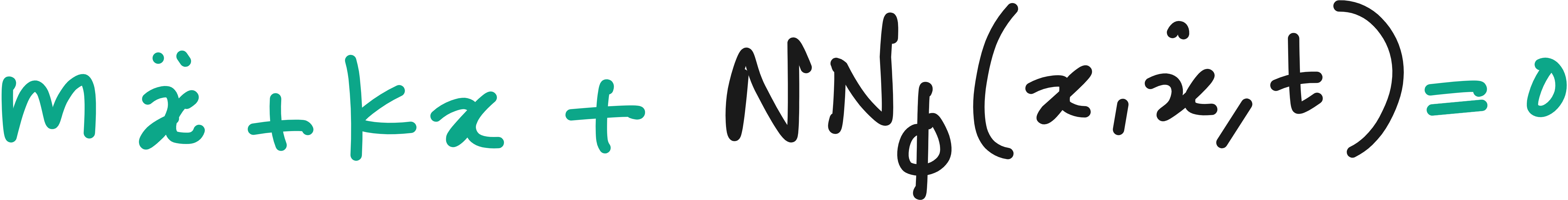
• Combine with the known ODE

  • The known part of the system is the classical second-order ODE, md^2x/dt^2+kx.

  • Instead of assuming a standard damping term c dx/dt, the model uses the neural network output Fd for damping.

  • So effectively, we have m d^2x/dt^2+kx+NNθ=0, where NNθ​ is the learned function.

• Numerical integration

  • With the neural network’s output inserted into the ODE, you integrate this hybrid equation forward in time- from t=0 (using the known initial condition) to each time point ti. You can perform the numerical integration using Runge Kutta method.

  • This gives a predicted trajectory for the entire time span.

• Compare predictions to experimental data

  • For each measured time ti, the predicted x is compared against the true data.

  • The loss function (often a sum of squared errors across all time points) measures how far the predicted trajectory is from the actual data.

• Back-propagation and optimization

  • The neural network parameters θ are adjusted (via gradient descent or similar optimizers) to minimize that loss.

  • Crucially, modern frameworks can differentiate through the numerical solver, making it possible to directly optimize θ based on how well the integrated ODE matches the observed data.

• Final model

  • Over many training epochs, the neural network converges to a damping function that best explains the data while still obeying the partial known physics.

  • The result is a Universal Differential Equation that reproduces the real system’s behavior more accurately than a purely known or purely data-driven model alone.

Lecture on UDE

I have made a lecture video on UDEs (meant even for absolute beginners) and hosted it on Vizuara’s YouTube channel. Do check this out. I hope you enjoy watching this lecture as much as I enjoyed making it.

Let us solve the spring + mass + unknown damper using UDE

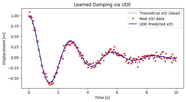
The below plots are the result of UDE implementation in Python.

• Red dots represent noisy measured data of the mass displacement over time.

• The dashed green line represents the ideal (theoretical) solution without any unknown damping.

• The solid blue line is the UDE model’s predicted displacement after learning the damping.

• We see that the blue prediction line tracks the noisy data points more accurately than the ideal solution, showing the model has learned the extra damping effect.

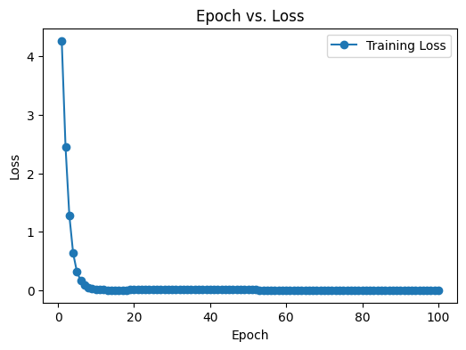
The loss plot below shows the loss (prediction error) rapidly decreasing from around 4 down to near 0 within the first few epochs, and then remaining low, indicating successful training of the neural network to capture the unknown damping.

By epoch 100, the blue curve closely follows the red data points, confirming the UDE has converged to a damping function that explains the observed motion more accurately.

After 100 epochs

Here is the Google Colab notebook with the full code: Link

Import libraries

import numpy as np
import matplotlib.pyplot as plt
from scipy.integrate import solve_ivp

Generate true data

# -----------------------------
# Step 1: Generate "true" data
# -----------------------------

# Physical parameters (assumed known in the real problem)
m = 1.0   # mass
k = 5.0   # spring constant

# "True" damping coefficient -- we pretend we don't know this!
c_true = 0.7

# Define the classical ODE for data generation
def damped_spring_mass(t, y):
    """
    y = [x, x_dot]
    returns dy/dt = [x_dot, x_ddot]
    """
    x, x_dot = y
    x_ddot = -(c_true/m)*x_dot - (k/m)*x
    return [x_dot, x_ddot]

# Initial conditions
x0 = 1.0    # initial displacement
v0 = 0.0    # initial velocity
y0 = [x0, v0]

# Time span for simulation
t_start, t_end = 0.0, 10.0
t_eval = np.linspace(t_start, t_end, 200)  # 200 time points

# Solve the classical ODE
sol = solve_ivp(damped_spring_mass, [t_start, t_end], y0, t_eval=t_eval)
x_true = sol.y[0, :]  # x(t)
v_true = sol.y[1, :]  # x_dot(t)

# Add noise to simulate experimental data
noise_level = 0.05
x_noisy = x_true + noise_level * np.random.randn(len(x_true))
v_noisy = v_true + noise_level * np.random.randn(len(v_true))

# Plot the noisy data vs. true solution
plt.figure(figsize=(8,4))
plt.plot(t_eval, x_true, label='Ideal $x(t)$')
plt.plot(t_eval, x_noisy, 'o', label='Real $x(t)$ data with noise', alpha=0.5, markersize=3)
plt.title("Simulated Data for a Damped Spring–Mass System")
plt.xlabel("Time [s]")
plt.ylabel("Displacement [m]")
plt.legend()
plt.show()

install torchdiffeq

pip install torch torchdiffeq

import torch packages

import torch
import torch.nn as nn
import torch.optim as optim
from torchdiffeq import odeint

Define the NN

# -----------------------------
# Step 2: Build the Neural Network
# -----------------------------

class DampeningNN(nn.Module):
    """
    A simple feed-forward neural network that takes:
      - current displacement u1,
      - current velocity u2,
      - optionally time t,
    and outputs an estimate of the 'damping force' (or part of it).
    """
    def __init__(self, input_dim=2, hidden_dim=16):
        super(DampeningNN, self).__init__()

        # You can include time as input (then input_dim=3)
        # For simplicity, we only use (u1, u2) => input_dim=2
        self.net = nn.Sequential(
            nn.Linear(input_dim, hidden_dim),
            nn.Tanh(),
            nn.Linear(hidden_dim, hidden_dim),
            nn.Tanh(),
            nn.Linear(hidden_dim, 1)  # output is a single value for damping
        )

    def forward(self, t, u):
        # u is (batch_size, 2) -> [x, x_dot]
        # t is a scalar or shape (batch_size, )
        # We'll just ignore t for now, or we could incorporate it
        return self.net(u)

Define the UDE

# -----------------------------
# Step 3: Define the UDE ODE function
# -----------------------------

class SpringMassUDE(nn.Module):
    """
    This class wraps the ODE:  du1/dt = u2
                               du2/dt = -(k/m)*u1 - (1/m)*NN(u1,u2)
    """
    def __init__(self, m, k, nn_model):
        super(SpringMassUDE, self).__init__()
        self.m = m
        self.k = k
        self.nn_model = nn_model  # the neural network for damping

    def forward(self, t, y):
        """
        y: [u1, u2]
        returns dy/dt
        """
        u1, u2 = y[..., 0], y[..., 1]  # shape: (batch_size,) if batch ODE
        # Reshape or combine for feeding the NN
        u_cat = torch.stack([u1, u2], dim=-1)  # shape: (batch_size, 2)

        # Damping force from NN
        damp_force = self.nn_model(t, u_cat)  # shape: (batch_size, 1)
        damp_force = damp_force.squeeze(dim=-1)  # make it (batch_size,)

        # The ODE:
        du1dt = u2
        du2dt = - (self.k / self.m) * u1 - (1.0 / self.m) * damp_force

        return torch.stack([du1dt, du2dt], dim=-1)

Convert our numpy arrays to PyTorch tensors

# Convert our numpy arrays to PyTorch tensors
t_train_torch = torch.tensor(t_eval, dtype=torch.float32)  # shape (N,)
x_train_torch = torch.tensor(x_noisy, dtype=torch.float32) # shape (N,)
v_train_torch = torch.tensor(v_noisy, dtype=torch.float32) # shape (N,)

Forward simulation

def forward_sim(net_ode, y0, t_points):
    """
    net_ode: an instance of SpringMassUDE
    y0: initial condition, shape (2,)
    t_points: 1D tensor of time points at which we want the solution
    returns: solution at those time points, shape (len(t_points), 2)
    """
    # We use odeint from torchdiffeq
    y0_torch = y0.unsqueeze(0)  # shape (1, 2) for batch dimension
    sol = odeint(net_ode, y0_torch, t_points, method='rk4')
    # sol shape is (len(t_points), batch_size=1, 2)
    return sol[:, 0, :]  # remove batch dim -> shape (len(t_points), 2)

Instantiate neural network and UDE

# Instantiate neural network and UDE
hidden_dim = 16
damping_nn = DampeningNN(input_dim=2, hidden_dim=hidden_dim)
ude = SpringMassUDE(m=m, k=k, nn_model=damping_nn)

# Initial condition for training
y0_torch = torch.tensor([x_noisy[0], v_noisy[0]], dtype=torch.float32)

# Choose an optimizer
optimizer = optim.Adam(ude.parameters(), lr=1e-2)

# 1) Create a list to store losses over epochs
loss_history = []


# We'll define a simple training loop
num_epochs = 20
print_interval = 5

for epoch in range(num_epochs):
    optimizer.zero_grad()

    # Forward simulation from t_start to t_end
    sol_pred = forward_sim(ude, y0_torch, t_train_torch)
    # sol_pred shape = (N, 2), where N = len(t_eval)
    x_pred = sol_pred[:, 0]
    v_pred = sol_pred[:, 1]

    # Define a loss: MSE on displacement (and optionally velocity)
    loss_x = torch.mean((x_pred - x_train_torch)**2)
    loss_v = torch.mean((v_pred - v_train_torch)**2)
    # Weighted sum or just x
    loss = 0.5*loss_x + 0.5*loss_v

    # Backprop
    loss.backward()
    optimizer.step()

    # Store the loss for plotting
    loss_history.append(loss.item())

    if (epoch+1) % print_interval == 0:
        print(f"Epoch {epoch+1}/{num_epochs}, Loss = {loss.item():.6f}")

# 3) Plot Epoch vs Loss
plt.figure(figsize=(6,4))
plt.plot(range(1, num_epochs+1), loss_history, marker='o', label='Training Loss')
plt.xlabel("Epoch")
plt.ylabel("Loss")
plt.title("Epoch vs. Loss")
plt.legend()
plt.show()

Final plots

# After training:
sol_final = forward_sim(ude, y0_torch, t_train_torch).detach().numpy()
x_final = sol_final[:, 0]
v_final = sol_final[:, 1]

plt.figure(figsize=(8,4))
plt.plot(t_eval, x_true, 'g--', label='True x(t) (ideal)', alpha=0.7)
plt.plot(t_eval, x_noisy, 'ro', label='Noisy x(t) data', markersize=3)
plt.plot(t_eval, x_final, 'b-', label='UDE Predicted x(t)')
plt.xlabel("Time [s]")
plt.ylabel("Displacement [m]")
plt.legend()
plt.title("Learned Damping via UDE")
plt.show()