
Modern Robot Learning Lecture 1 - Robot Imitation Learning
What is Imitation Learning and where is it used in modern robot learning?

Let us take a simple example:
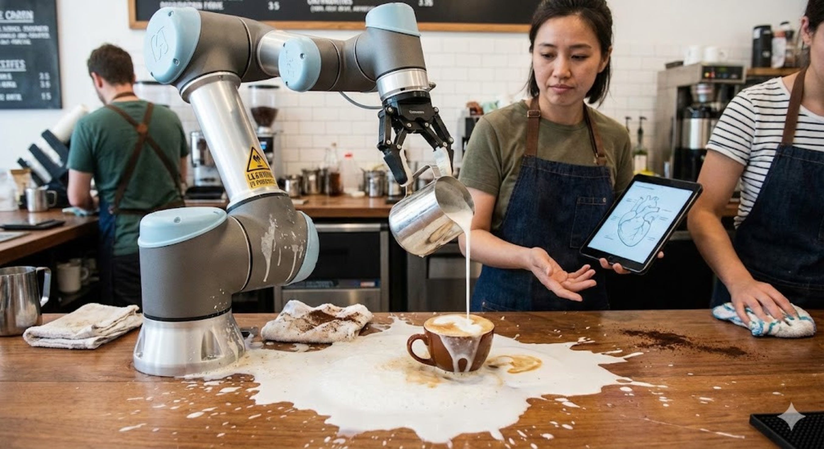
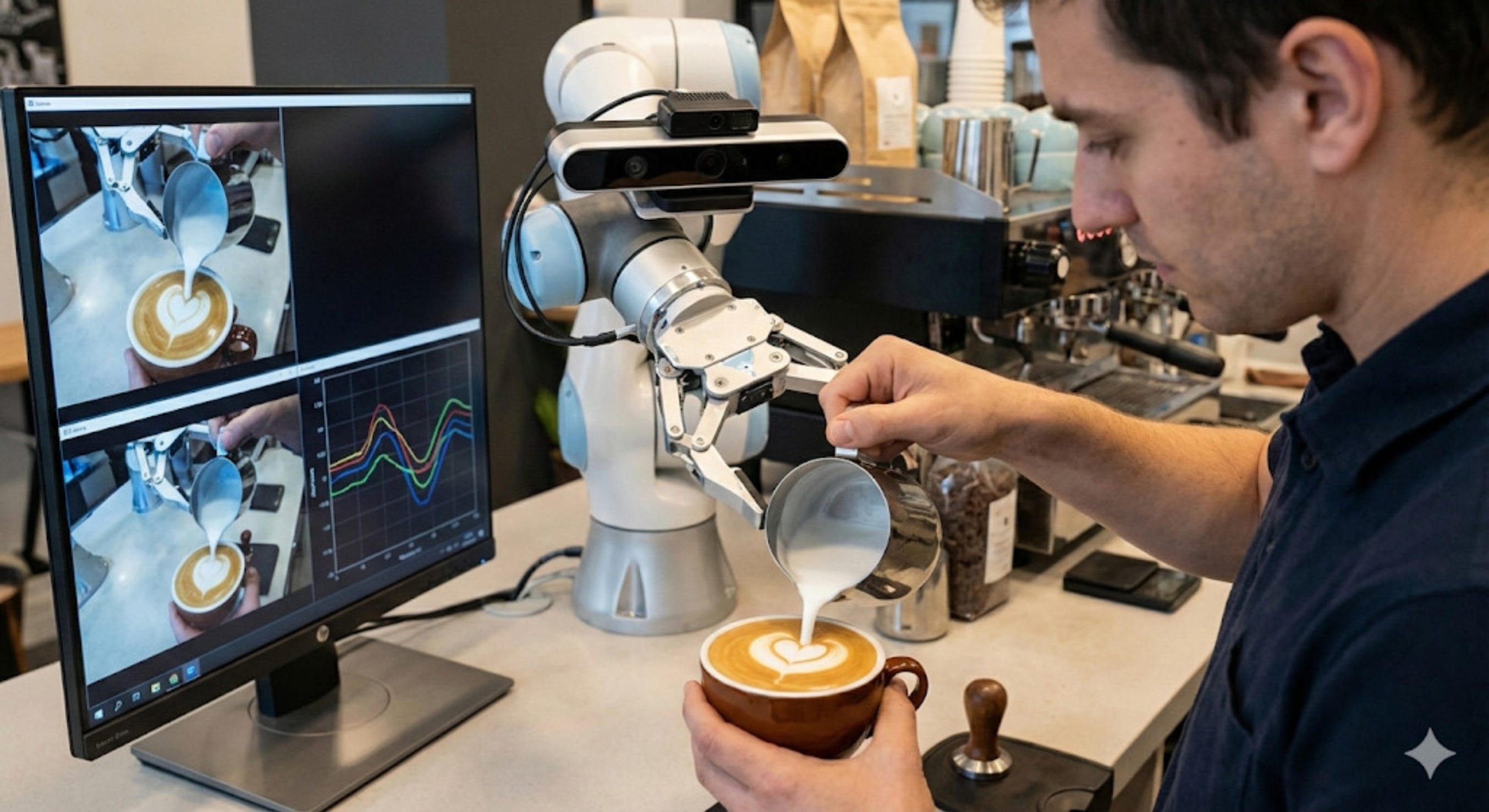
Suppose we want to train a robot to pour a “heart shape” in a coffee (latte)

Let us say we think of an approach where we will allow the robot to make mistakes and learn from them.
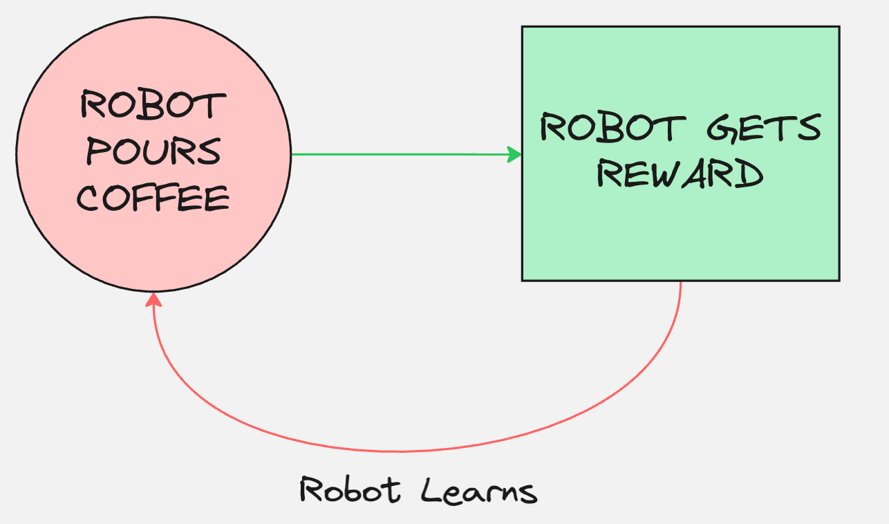
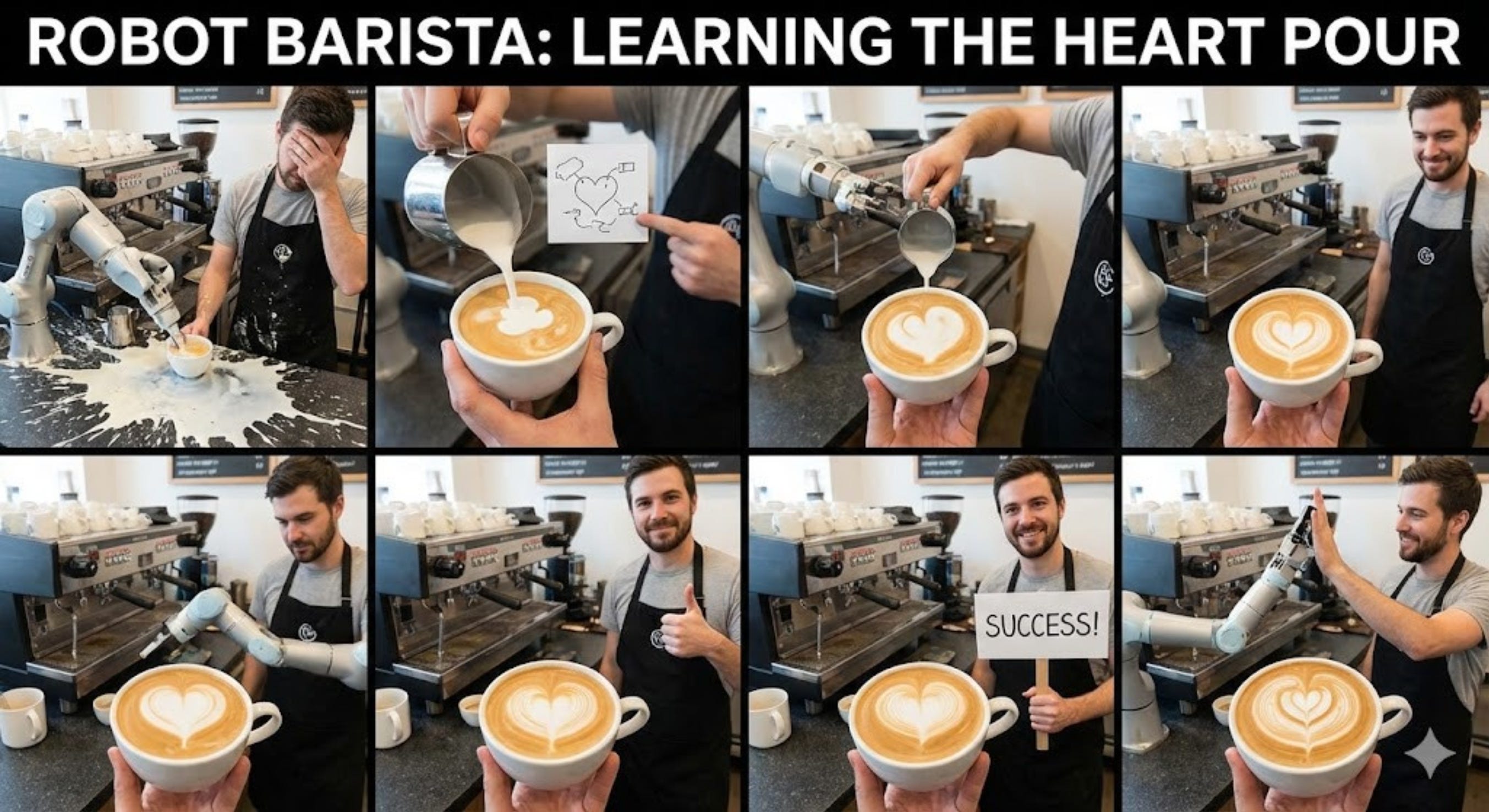
In this approach, the robot is bound to make mistakes when it starts.
So initially, the robot might start out with spilling the coffee outside the cup.
Slowly and steadily, the robot will learn from its mistakes. It will learn to increase its rewards. And finally, it will learn to pour the heart shape into the coffee latte.
This process is called reinforcement learning.
Reinforcement learning is a popular technique where the agent improves with time.
The objective of RL is to learn a policy such that for every state you predict an action which has the maximum expected reward in the future.
Then why not use RL for Robotics, why are we talking about Imitation Learning?
There are 3 major drawbacks of the Reinforcement Learning method:
Problem #1: The robot has to explore randomly at first. It will throw hot milk on the floor, smash the ceramic mug, or pour milk onto its own circuits.
This is what makes the exploration phase in reinforcement learning potentially costly and unsafe.
Problem #2: Every time it spills, a human has to clean the mess, refill the pitcher, and get a new mug. You cannot automate this reset process.
Problem #3: How do you write a mathematical function for a beautiful heart shape? Is it pixel density? Symmetry? It is incredibly hard to define a dense reward for artistic style.
All of these factors complicate training RL algorithms on hardware at scale.
Can you think of an alternative way of solving this problem?
What if the robot learnt from demonstrations?
Let us simplify the problem by considering the following: Suppose that the robot is fixed, and the only thing which is moving are the wrists of the robot.
Now, using the wrists, the robot is pouring coffee into a mug.
And we want to train the robot to successfully pour the coffee into the mug.
Now with this problem in mind, we can create the following dataset with a set of inputs and a set of outputs.
The inputs and the outputs look as follows:
Input: Wrist Angle at current time step
Output: Wrist Angle at next time step
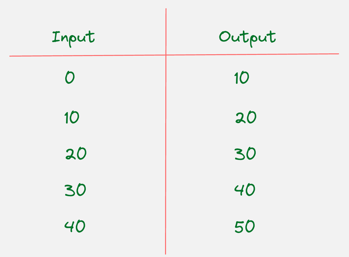
This can be shown in the following plot:
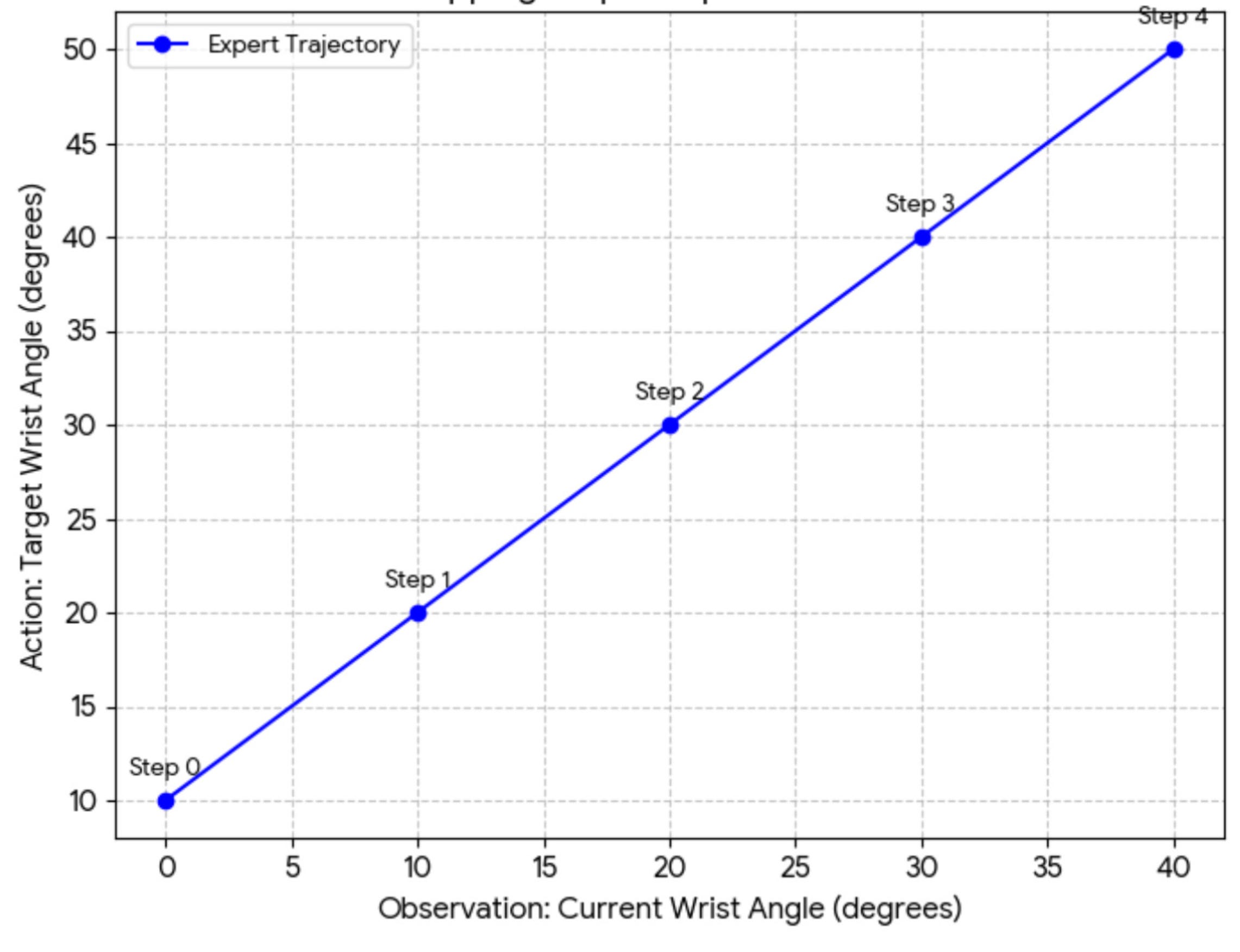
Notice that we have used the words “observations” and “actions” for the inputs and outputs, respectively. This is borrowed from the RL literature.
In this example, we have only considered the wrist angle as the observation. However, in reality, it could include all the joint angles that are there in the robot.
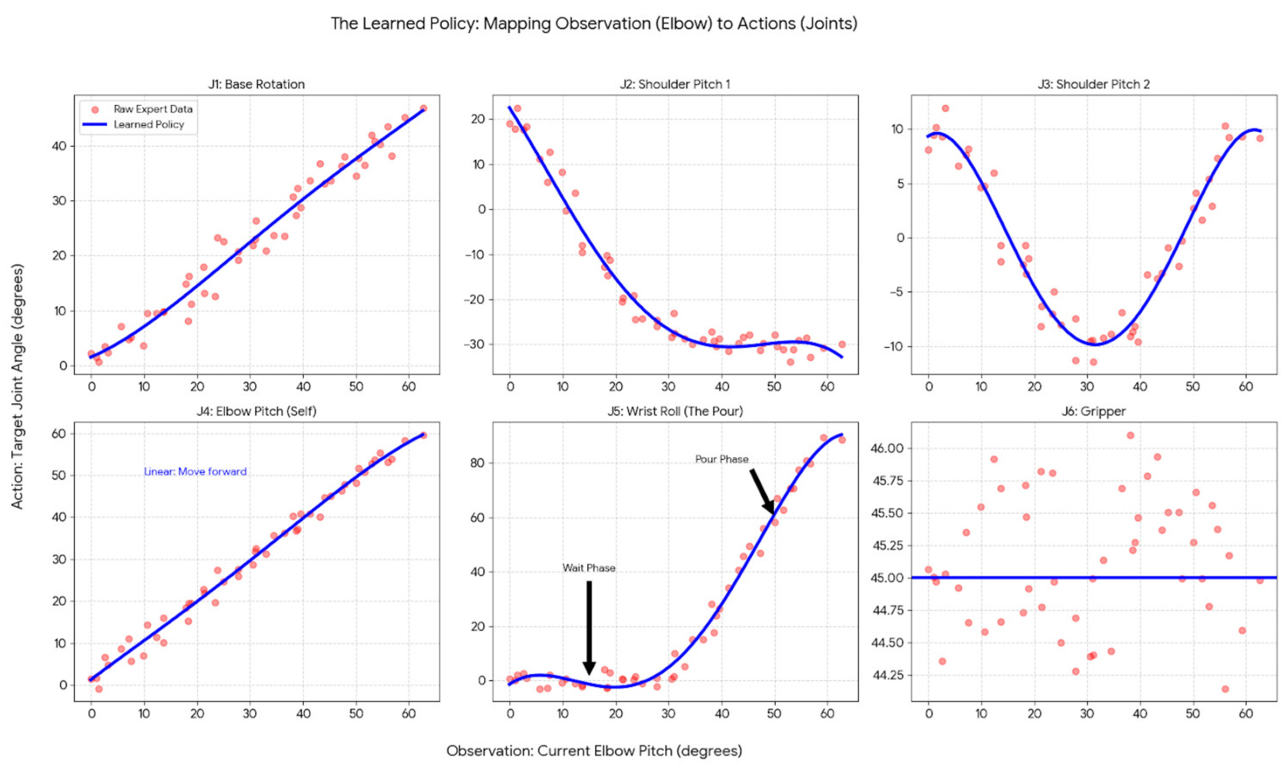
For example, for SO-101, let us understand how many joint angles are there:
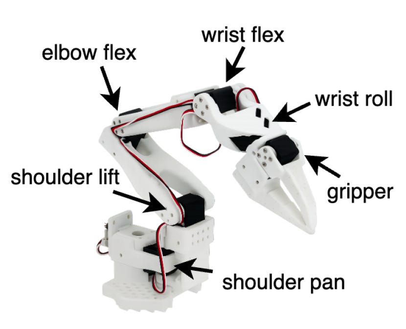
The SO-101 Arm has 6 degrees of freedom.
So now the input-output pairs will be created for six variables, which will look as follows:
Can you tell me what is wrong in the about diagram? What am I missing?
In the above figure, we have considered one input and 6 outputs.
Let us try to write down the input-output pairs mathematically:
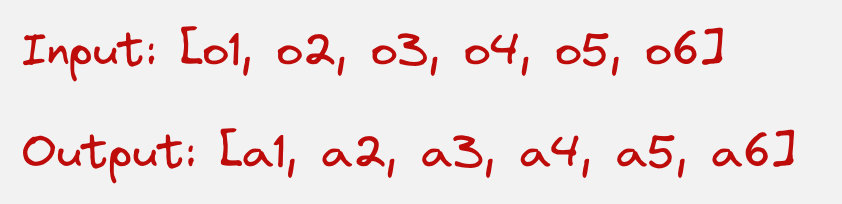
The input has six dimensions, and the output also has six dimensions.
Once we create the input-output pairs, our objective function is to design a model which can minimize the loss between the input and the output.
The model will take the six observations as input and outputs all actions. Humans cannot visualize a six-dimensional graph.
This is very similar to traditional supervised learning tasks in the field of machine learning.
The data about joint angles is also called proprioceptive data.
I was initially very confused where this word comes from, but it means your body’s subconscious sense of its own position, movement, and effort in space.
With this understanding, let us revisit our initial problem of pouring a heart shape in a latte.
Let us assume that we collect 100 expert demonstrations of humans collecting the jar and pouring the milk with the exact shape that we want.
So we have actually captured the entire proprioperceptive data.
Now let us assume that we train an ML model to understand the relation between the input and the output.
We have learned exactly how all the joints should move to achieve our goal.
Does that mean we are done?
What will happen if we move the cup towards the right of the location which is used for collecting the training data?

Since we have only captured the proprioceptive data, we will be able to move the joints in such a way that we are pouring a heart shape, but it will be poured in a completely different location.
This means that we need a camera to capture the image data as well!
“The robot needs visual data from a camera to perceive the world around it. Locate objects and adjust its actions accordingly to succeed”
For example, if we have a camera mounted on a SO101 robot, it will capture the images of the milk being poured into the coffee.
These images will be captured for all the time steps.
The final observations, thus consist of a combination of the proprioperceptive data and the visual data.
This can be visually understood with the help of the schematic below:
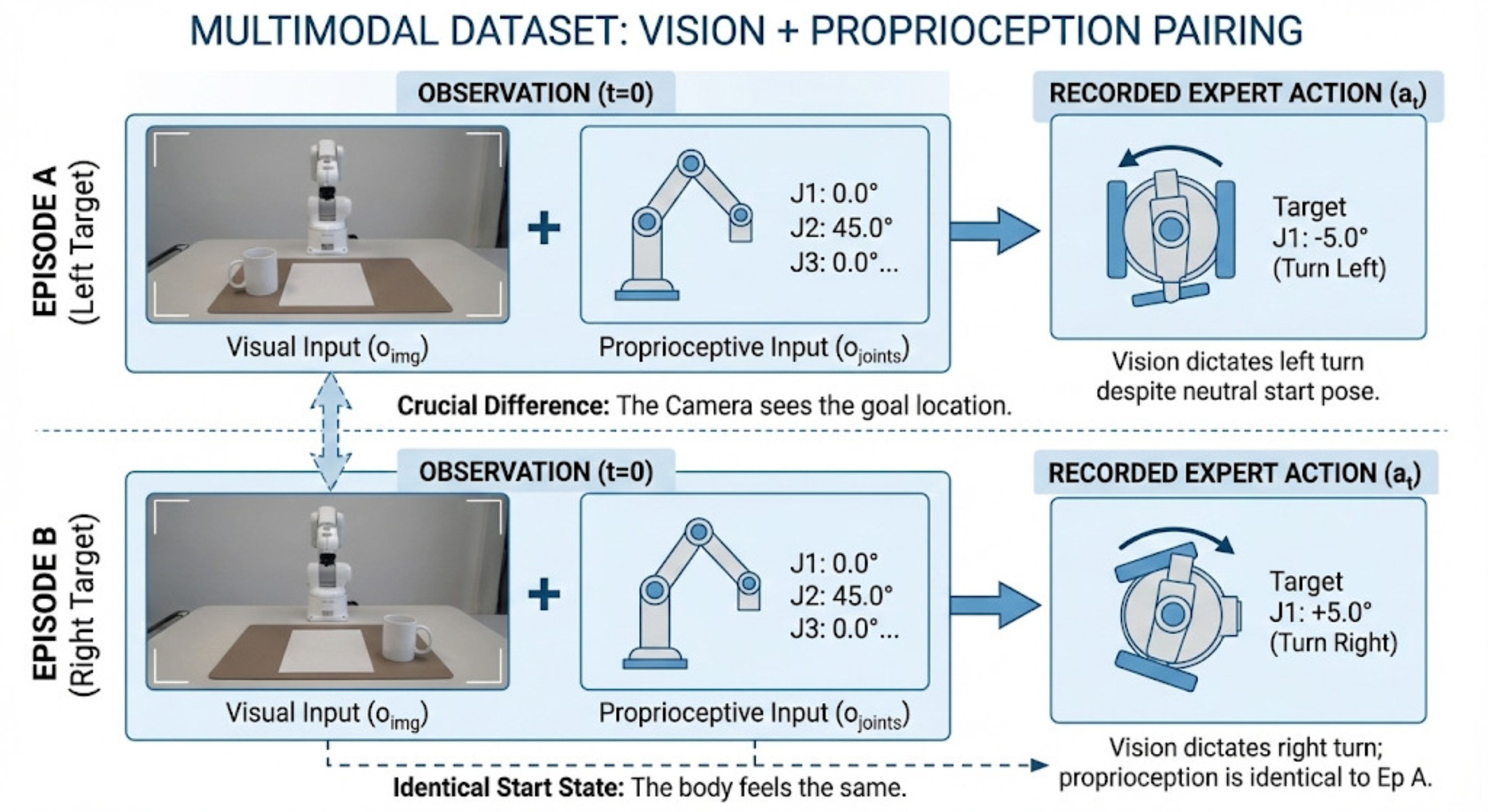
So the dataset becomes multi-modal.
Let us take some actual examples to make this clear.
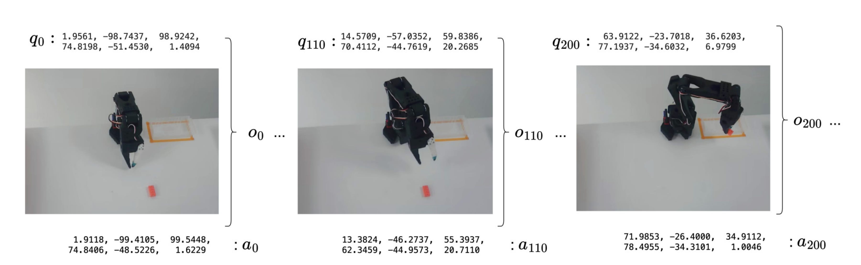
These are some sample observations and action pairs over the course of a given trajectory which is recorded in a sample dataset in the LeRobot library.
Let us look at an actual dataset!

Now, can we try to think of the advantages which imitation learning offers over reinforcement learning?
Training happens offline and from expert human demonstrations. This prevents the robot from performing dangerous actions.
Reward design is entirely unnecessary, as demonstrations already reflect human intent.
Expert trajectories encode terminal conditions, success detection and resets are implicit in the dataset.
Empirical evidence suggests the performance of Imitation Learning scales naturally with growing corpora of demonstrations collected across tasks, embodiments, and environments.
If imitation learning is so great, then we can simply record human demonstrations of the specific task and allow the robot to learn from them. What is the problem with the above approach?
Note that, here we are mapping observations to actions. These are called point estimate policies.
To understand the limitations of point estimate policies, let us look at a specific example:
Let us consider a scenario:
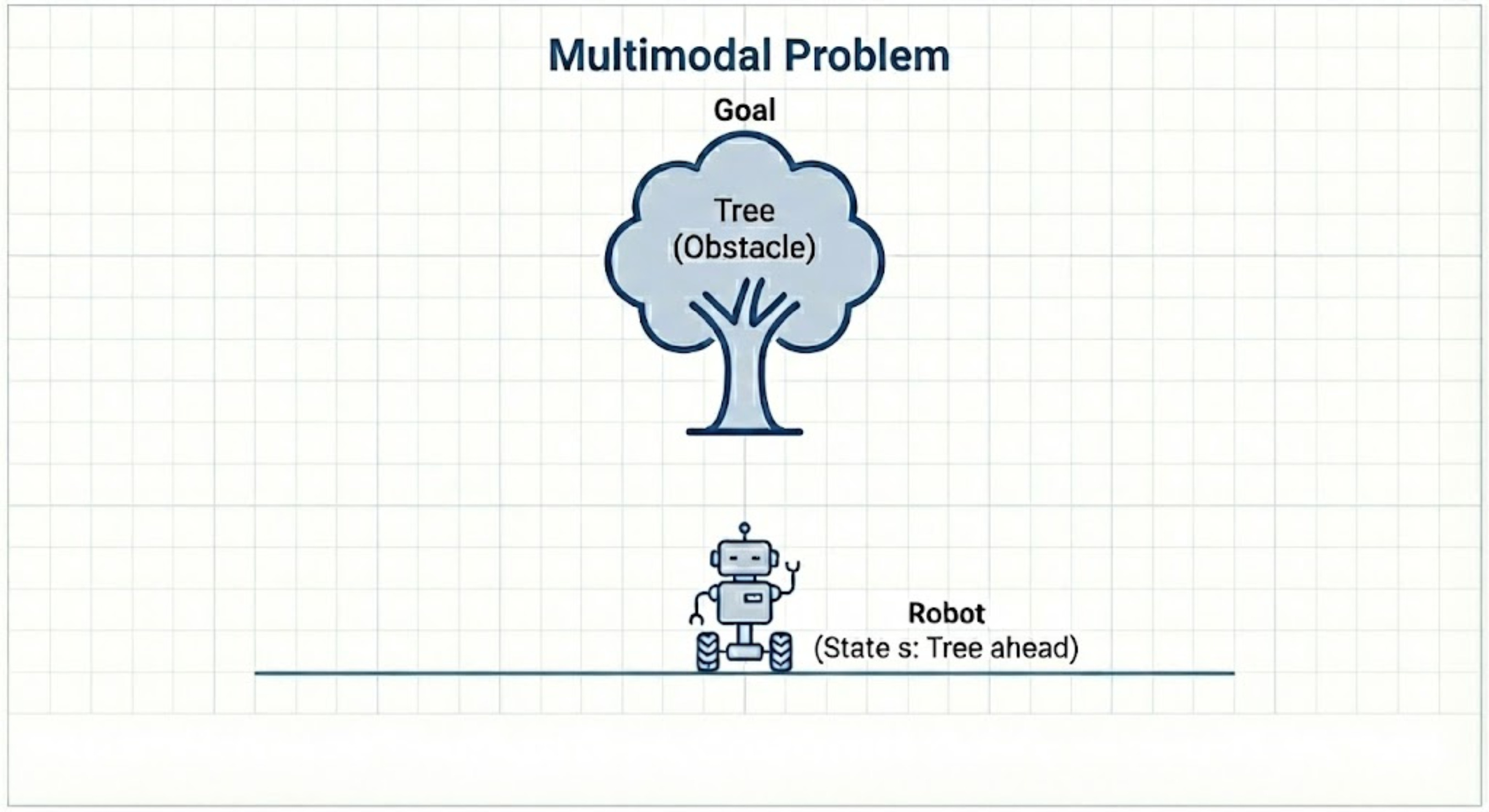
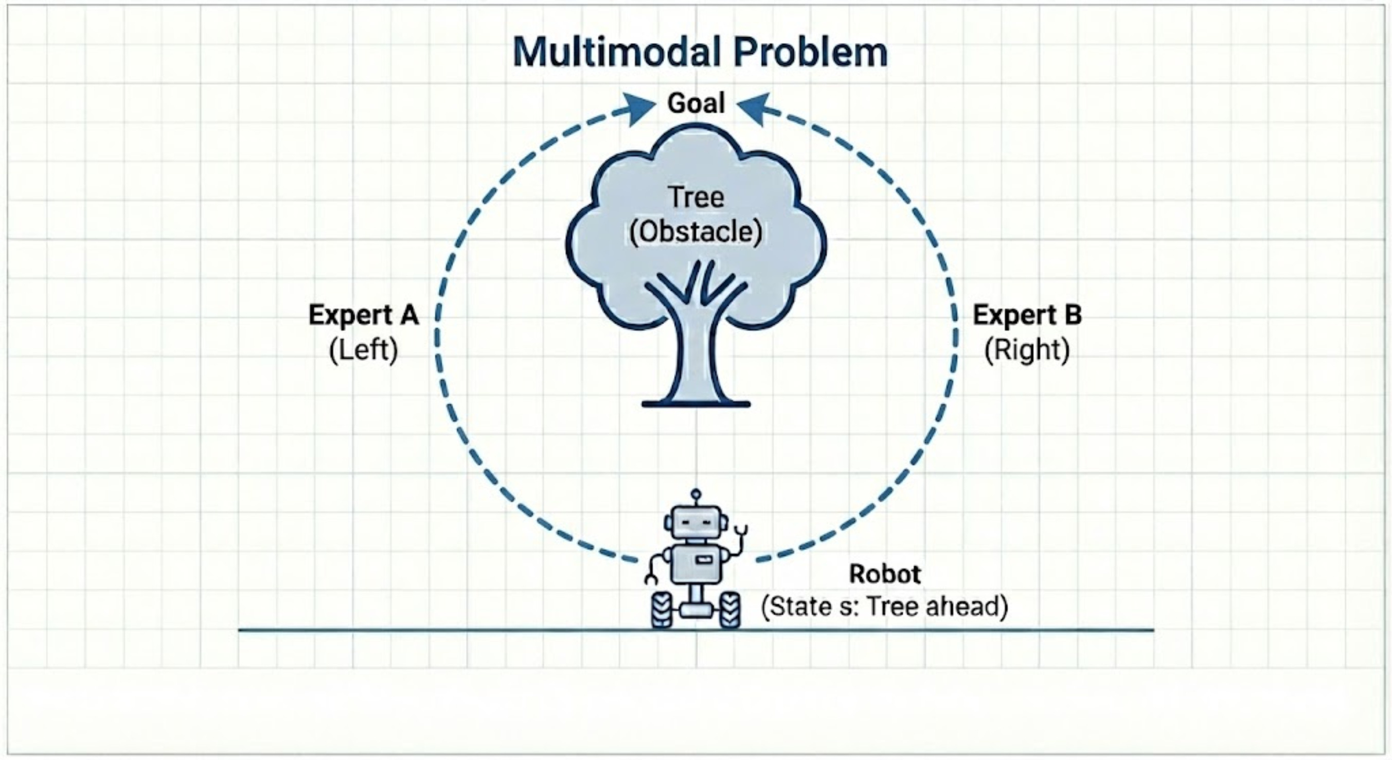
Imagine you are training a robot to navigate a path. It has a camera (its “state”) and can steer left or right (its “action”).
The path is such that there is an obstacle in the path, like a large tree, and you have to navigate. You have to train a robot to go around the obstacle and reach the goal.
It looks something like this:
In the first step, you are collecting the data. The data is collected by recording trajectories controlled by a human expert.
Now a human expert can navigate the robot in any way. Let us assume that there are two data points recorded by the human expert:
Data point A: The expert sees the tree and steers left to go around it. This is a perfectly valid successful action.
Data point B: Later the expert sees the exact same tree but decides to steer right to go around it. This is also a perfectly valid successful action.
Now, you try to train a simple supervised learning model on this data.
The model’s goal is to find a single function that predicts the action from the state.
It works by minimizing the error between its prediction and all the expert’s actions.
The model sees that for the state “tree ahead,” the answers are sometimes “steer left (-1)” and sometimes “steer right (+1)”.
To minimize its total error across all these examples, the model finds the mathematical average of the expert’s actions.
The average of “steer left” and “steer right” is “steer straight ahead (0)”.
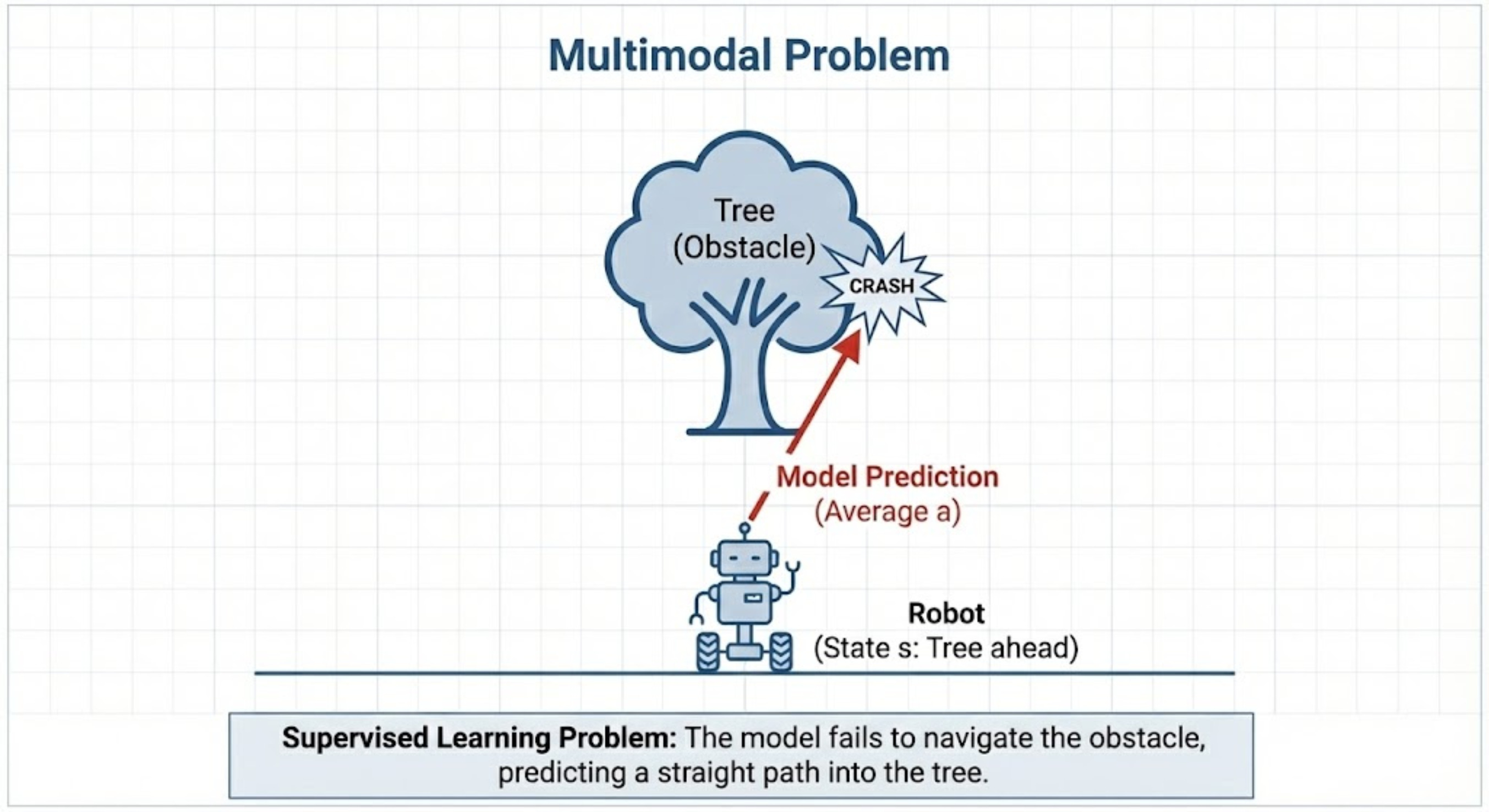
We call this a multi-modality problem because if it happens that for the same state, there are more than one actions, then the model takes the average of those actions as the real behavior.
This can be visually seen through the following graph:
What we ideally want is that for every state, we want to learn the distribution of all possible actions, not the average.
“Point-estimate policies typically fail to learn multimodal targets, which are very common in human demonstrations solving real-world robotics problems, as multiple trajectories can be equally as good towards the accomplishment of a goal”
Another example is shown below:
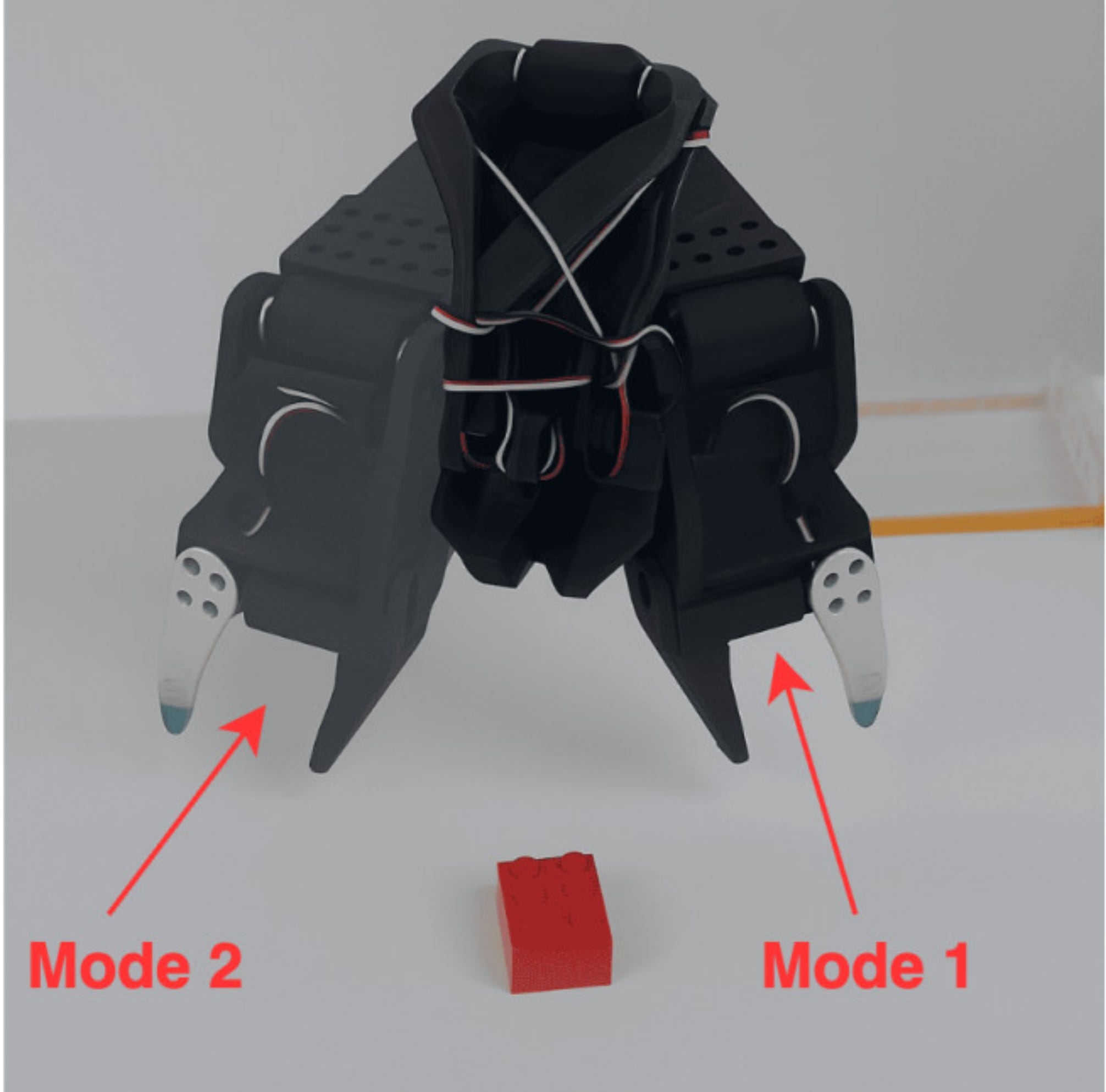
The task given for the human demonstrations is to pick the object which is shown in red.
The robot can either go left or right to pick this object. So here also, we will have multi-modal demonstrations in the dataset.
Let us look at a practical example:
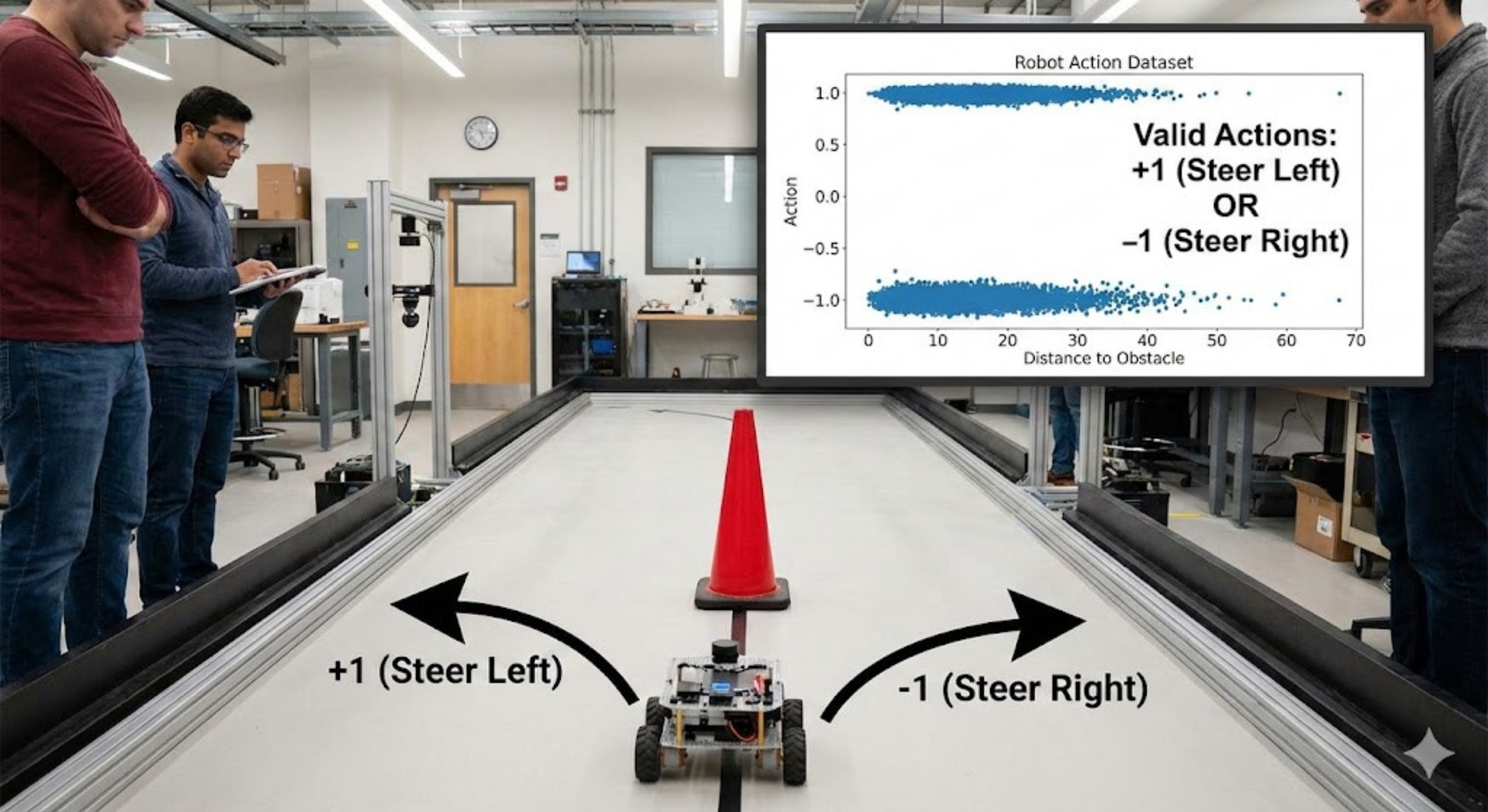
Objective: The robot has to steer left or right to cross the pole
Expert humans record demonstrations to achieve this task. Some of them steer the robot left, and some of them steer the robot right.
We want to demonstrate through this example how point-estimate policies fail in robotics.
Here is the Google Colab code which we use to illustrate this:
Why do Point Estimate Policies Fail in Robotics - Code
(Refer to the code file - Lecture 1 - Robot Imitation Learning.ipynb)
Here is the final graph which we get:
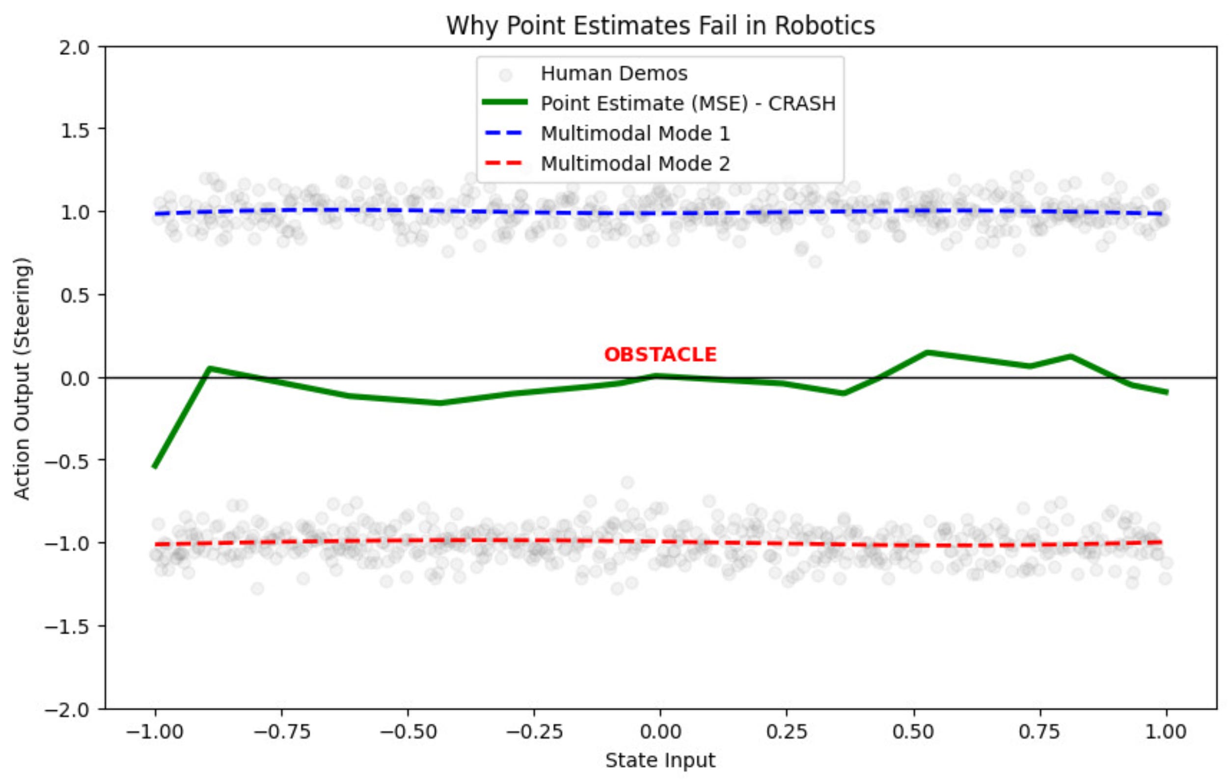
Closely observe from this graph that the point estimate (shown in green) hits the obstacle.
This provides a very strong argument as to why we need policies which capture the distribution of the data.
In the next lecture, we will cover deep generative modeling and how it can solve the multi-modal problem in the robotics.
If you like this content, please check out our bootcamps on the following topics:
Modern Robot Learning: https://robotlearningbootcamp.vizuara.ai/
GenAI: https://flyvidesh.online/gen-ai-professional-bootcamp
RL: https://rlresearcherbootcamp.vizuara.ai/
SciML: https://flyvidesh.online/ml-bootcamp