
Knowledge Distillation & Data-Efficient Image Transformers
The original ViT needed 300 million images to outperform CNNs. DeiT does it with just 1.2 million, by letting a CNN teacher distill its visual intuitions into a transformer student.

This chapter covers
Understanding inductive biases in CNNs and why they matter for image understanding
Why Vision Transformers are data-hungry and computationally expensive without these biases
How DeiT (Data-efficient Image Transformers) achieves competitive accuracy using only ImageNet-1K
The mechanics of knowledge distillation, from soft labels to dark knowledge
The mathematics behind temperature scaling, KL divergence, and DeiT’s loss functions
Building a complete DeiT implementation from scratch in PyTorch
Data Efficient Image Transformer Code is available below
https://github.com/VizuaraAI/Transformers-for-vision-BOOK
[Don't forget to star the code repo!]
In previous blog, we explored how Vision Transformers (ViTs) brought the power of self-attention to computer vision by splitting images into patches and processing them as sequences. The results were remarkable: ViT achieved state-of-the-art accuracy on ImageNet. But there was a catch. That performance came at an enormous cost. The original ViT required pre-training on JFT-300M, a private Google dataset containing 300 million labeled images, and demanded thousands of TPU-days of compute. For most researchers and practitioners, this was simply out of reach.
In this blog, we will explore how DeiT (Data-efficient Image Transformers) solved this problem. Published by Touvron et al. from Facebook AI Research and Sorbonne University in 2021, DeiT achieved competitive accuracy using only ImageNet-1K (1.2 million images), which is 250 times less data than the original ViT required. The key insight was combining a clever training recipe with knowledge distillation, a technique where a smaller student model learns from a larger, pre-trained teacher model. But before we dive into DeiT itself, we need to understand why Vision Transformers struggle with limited data in the first place. The answer lies in a concept called inductive bias.
Prerequisites blogs


1.1 Inductive bias: the built-in assumptions of neural networks
When we train a neural network, we are asking it to learn patterns from data. But no model starts from a completely blank slate. Every architecture carries certain built-in assumptions about how data is structured, and these assumptions shape what the model finds easy or difficult to learn. These built-in assumptions are called inductive biases.
Think of it this way: if you were asked to find a lost cat in a neighborhood, you would naturally check under porches, in gardens, and near food sources. You would not start by searching the sky or underwater. Your prior knowledge about where cats tend to be gives you a huge advantage. You are not starting from scratch. Inductive bias works the same way for neural networks: it encodes structural assumptions that guide learning in the right direction, reducing the amount of data needed to reach good performance.
What are the inductive biases in CNNs?
Convolutional Neural Networks (CNNs) have two powerful inductive biases built directly into their architecture: locality and translation equivariance. Let us examine each in detail.
Locality bias. CNNs assume that nearby pixels are more related to each other than distant pixels. This assumption is enforced by the small convolutional filters (typically 3x3 or 5x5) that examine only a local patch of the image at each step. The network processes the image by looking at small neighborhoods first, detecting low-level features like edges and textures, and then gradually combining these local features into higher-level concepts through deeper layers. An edge detector in the first layer might find horizontal lines. The next layer combines several edges into a corner or a curve. Deeper layers assemble these parts into recognizable shapes like eyes, wheels, or letters.
This hierarchical, local-to-global processing mirrors how natural images are actually structured. In a photograph, a pixel showing part of a dog’s ear is highly correlated with neighboring pixels that also show the ear, but has little direct relationship with a pixel in the far corner showing a blade of grass. CNNs exploit this statistical property by design.
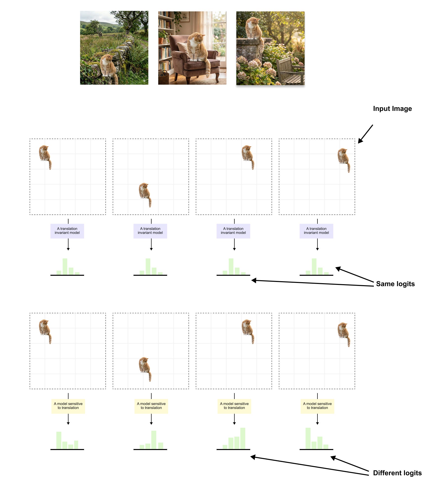
Figure 1.1: The effect of inductive bias on translation handling. Top: a cat is placed at four different positions within the input grid. A translation invariant model (CNN) produces the same logits every time, correctly recognizing the cat regardless of where it appears. This is because weight sharing and pooling are built into the architecture. Bottom: the same cat at different positions is passed through a model sensitive to translation (such as a ViT trained on limited data), which produces different logits for each position. The CNN does not need to learn that position should not affect the classification; this property is baked into its design. A ViT must discover this from data, which is why it requires far more training examples.
Translation equivariance.
The second key inductive bias is translation equivariance, a CNN detects the same feature regardless of where it appears in the image. This property comes from weight sharing , where the same convolutional filter is applied identically at every spatial position. Mathematically, f is a convolution operation and T is a spatial translation, then:
This means that if an object shifts position in the input, the corresponding feature map shifts by exactly the same amount. A cat-ear detector will fire whether the ear appears in the top-left corner or the bottom-right corner of the image. Figure 1.2 shows two concrete examples: the same convolutional kernel slides over the entire input and detects the same pattern wherever it occurs, whether that is a left edge in a grid of circles or a car on a road versus on a building rooftop.
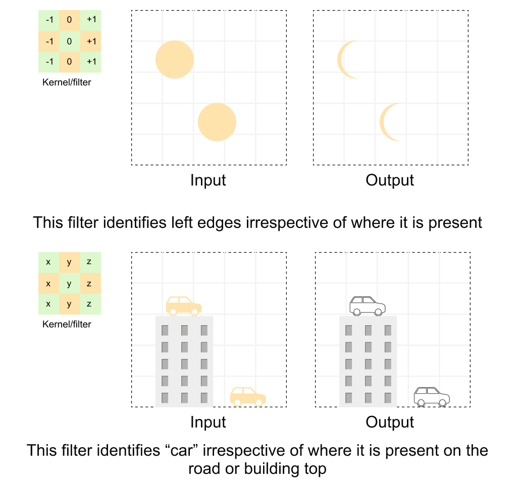
Figure 1.2: Translation equivariance in convolutions Top: a convolutional kernel (shown on the left) is applied across an input grid containing circles at different positions. The filter identifies left edges irrespective of where they appear in the input, producing the same edge-detection response in the output. Bottom: the same principle applied to a real-world scene. The kernel identifies “car” features regardless of whether the car is on the road or on a building rooftop. Because the same filter weights are shared across all spatial positions, the network does not need to learn separate detectors for every possible location of a feature. (conceptual illustration)
When we add pooling layers (max pooling or global average pooling) on top of convolutions, we achieve translation invariance: the final classification output remains the same regardless of where the object appears. The pooling operation discards precise positional information, summarizing each region with a single statistic (maximum or average value). This is why a CNN classifies an image as "cat" whether the cat is centered, shifted left, or shifted right.
NOTE
Translation equivariance and translation invariance are related but distinct properties. Equivariance means "the output shifts with the input" (convolution layers). Invariance means "the output stays the same regardless of position" (achieved after pooling). A CNN is equivariant through its convolutional layers and becomes invariant at its classification output through pooling.
Why are these biases so powerful?
These inductive biases are powerful precisely because they match the statistical structure of natural images. Consider what they give us:
Fewer parameters. Weight sharing means one small filter is reused across the entire image, rather than learning separate weights for every position. A 3x3 filter on 3 channels has only 27 parameters, yet it processes every location in the image.
Better generalization with less data. Because the model already “knows” that patterns can appear anywhere and that local neighborhoods matter, it does not need millions of examples to discover these facts.
Natural feature hierarchies. The local-to-global processing pipeline naturally builds the kind of part-based representations that are useful for recognition: edges combine into textures, textures into parts, parts into objects.
This is exactly why CNNs dominated computer vision for nearly a decade, from AlexNet in 2012 through the ResNet era. The built-in assumptions aligned beautifully with the task.
When do these biases become a limitation?
However, the same rigid assumptions that make CNNs data-efficient can become a ceiling on performance. Consider the image in figure 1.3: a person walking near a traffic signal. To understand this scene, the model needs to relate the person (in one part of the image) to the traffic signal (in a completely different part). These two elements are spatially far apart, but semantically they are deeply connected: the traffic signal determines whether the person should walk or stop.
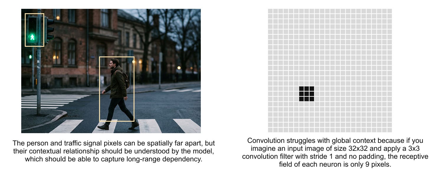
Figure 1.3 Long-range dependencies in images. The person and the traffic signal are spatially far apart in pixel space, but they are semantically related. A CNN must stack many layers to connect these distant regions through its limited local receptive field. A transformer, with global self-attention, can relate these elements directly in a single layer.
A CNN's local filters can only see a small neighborhood at each layer. To connect the person and the traffic signal, information must propagate through many layers, each expanding the receptive field slightly. By the time the model can "see" both elements simultaneously, the information has passed through many transformations and may be diluted or lost.
This is where transformers shine. Self-attention computes relationships between all patches simultaneously, regardless of spatial distance. A transformer can directly attend from the "person" patch to the "traffic signal" patch in a single layer. As we discussed in the context of natural language processing, this is analogous to how attention connects distant words in a sentence.
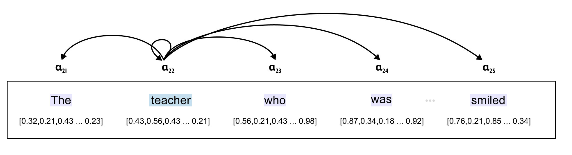
Figure 1.4 Attention mechanisms connect distant elements directly. Just as attention in NLP allows the word "smiled" to attend strongly to "teacher" despite the intervening words, visual attention allows distant image patches to interact directly. The attention weights (shown below the sentence) indicate how strongly each word attends to others, capturing long-range dependencies that local convolutions would struggle with.
So, inductive bias in CNNs is a double-edged sword. When the assumptions match the data (local features, translation-invariant patterns, moderate image complexity), CNNs are remarkably efficient. When the task demands flexible, global reasoning across distant image regions, those same assumptions become a constraint. This trade-off is precisely what motivated the development of Vision Transformers, and subsequently, DeiT.
1.2 Why Vision Transformers are data-hungry and computationally heavy
Now that we understand what inductive biases are and why CNNs benefit from them, we can understand the fundamental challenge that Vision Transformers face.
The ViT paper’s stark finding
The original Vision Transformer paper by Dosovitskiy et al. (2020) contained an important admission that is easy to overlook:
"We note that Vision Transformer has much less image-specific inductive bias than CNNs. In CNNs, locality, two-dimensional neighborhood structure, and translation equivariance are baked into each layer throughout the whole model. In ViT, only MLP layers are local and translationally equivariant, while the self-attention layers are global."
The paper continued with a crucial finding:
“Transformers do not generalize well when trained on insufficient amounts of data.”
Let us unpack exactly why. A Vision Transformer processes images very differently from a CNN:
No locality constraint. In every transformer layer, each patch attends to every other patch through self-attention. There is no architectural constraint forcing the model to prioritize nearby patches. The attention mechanism computes pairwise relationships between all patches simultaneously, whereas CNNs restrict each layer to local neighborhoods.
No weight sharing across positions. Unlike CNNs where the same filter slides across the entire image, in ViTs the attention mechanism can learn different relationships for different positions. Positional information comes only from learned positional embeddings, not from the architecture itself.
No hierarchical feature extraction by default. CNNs naturally build hierarchical features (edges, then textures, then parts, then objects) through stacked local convolutions with increasing receptive fields. Standard ViTs have uniform global attention at every layer, so this hierarchy must be learned entirely from data.
The data requirements
The consequence is stark. Since a ViT must learn locality, translation patterns, and hierarchical feature extraction all from scratch, it needs vastly more data.
The original ViT paper systematically studied this relationship with a dataset scaling experiment:
ImageNet-1K (~1.2 million images): ViT-Large underperforms comparable CNNs. Worse, larger ViT variants perform worse than smaller ones due to overfitting. The model memorizes training data rather than generalizing.
ImageNet-21K (~14 million images): ViT-Large and comparable CNNs perform similarly. The ViT begins to show its potential.
JFT-300M (~303 million images): ViT-Large significantly outperforms comparable CNNs. The pattern reverses completely: larger models perform better, not worse.
This reveals a fundamental trade-off in machine learning: the less prior knowledge (inductive bias) you build into an architecture, the more data it needs to learn those patterns from experience. CNNs “know” about locality and translation equivariance before seeing a single training image. ViTs must discover these properties purely from data, and discovering them requires seeing hundreds of millions of examples.
Scaling laws and the bitter lesson
This phenomenon connects to a broader principle in deep learning captured by scaling laws. Research by Kaplan et al. (2020) established that neural network performance follows predictable power-law relationships with three variables: model size (N parameters), dataset size (D tokens or images), and compute budget (C FLOPs):
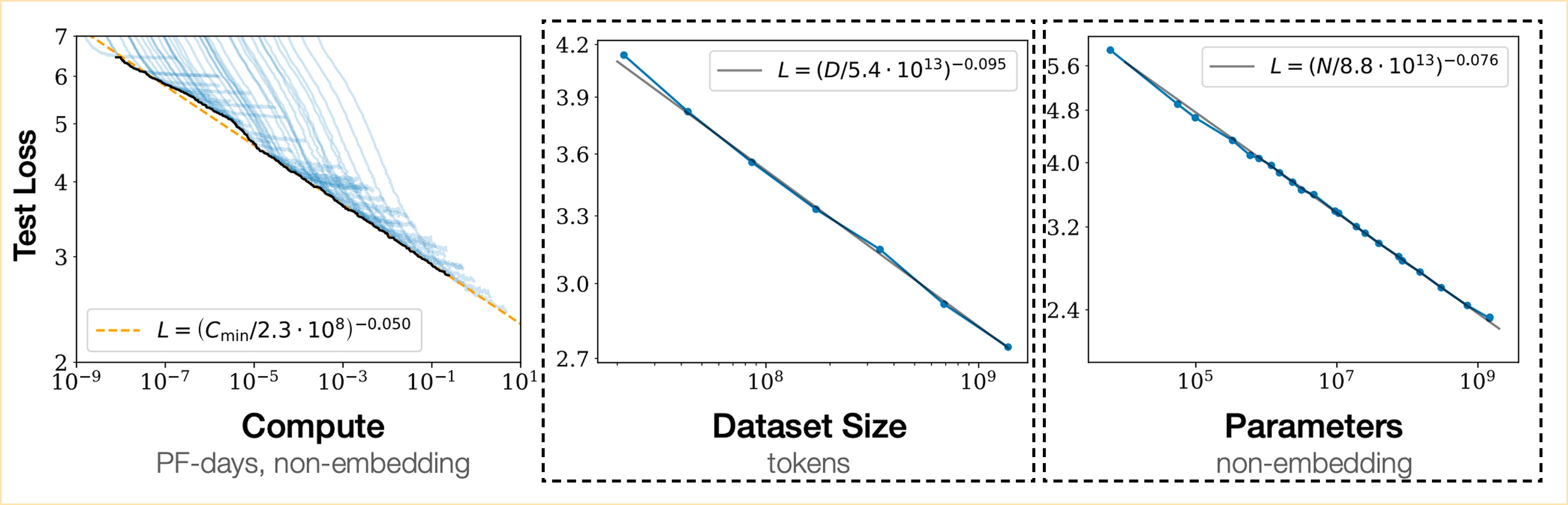
Figure 1.5 Scaling laws demonstrate that model performance improves as a smooth power law of model size, dataset size, and compute budget. These relationships, first established for language models, were later confirmed for Vision Transformers as well. The declining curves show that each doubling of resources yields a predictable (though diminishing) improvement in performance.
The Scaling Vision Transformers paper by Zhai et al. (2022) confirmed that these same power-law relationships hold for ViTs, scaling from 5 million to 2 billion parameters. The key insight is that architectural details matter less than scale. With enough data and compute, the flexibility of transformers (their lack of restrictive inductive biases) becomes an advantage rather than a limitation. The ViT paper itself summarized this as: “Large-scale training trumps inductive bias.”
But this raised an uncomfortable question: what if you do not have 300 million images and thousands of TPU-days? What if you have a single machine, a standard dataset, and a few days of training time? This is precisely the problem that DeiT set out to solve.
The small context window insight
Consider how a small local patch of an image can be ambiguous without global context. Figure 1.6 shows an interesting property: small context windows of different digits can look remarkably similar. The bottom halves of the digits 8, 0, and 6 share nearly identical local features. A local convolutional filter might struggle to distinguish them, while global attention can consider the entire digit.
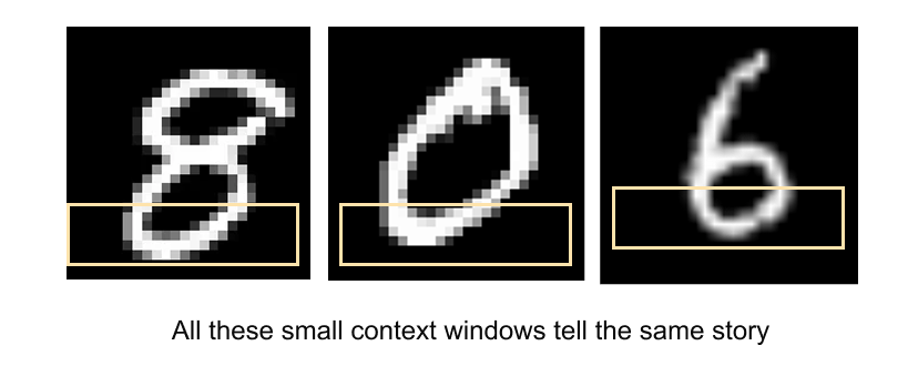
Figure 1.6 Small context windows can be ambiguous. The bottom portions of the digits 8, 0, and 6 appear nearly identical when viewed in isolation. This illustrates both the strength and weakness of local processing: CNNs capture these shared local features efficiently, but transformers with global attention can disambiguate by considering the full spatial context simultaneously.
This is a microcosm of the broader tension between CNNs and ViTs. Local processing is efficient but can miss the forest for the trees. Global processing is powerful but expensive to learn. DeiT’s genius was finding a way to get the best of both worlds.
1.3 DeiT: data-efficient training through distillation
With the problem clearly defined (ViTs need too much data and compute), let us explore how DeiT solved it. The paper “Training data-efficient image transformers & distillation through attention” by Touvron et al. (2021) introduced a remarkably elegant solution that combines two key ingredients: a carefully designed training recipe and a novel form of knowledge distillation.
The core idea
DeiT’s central insight is this: instead of requiring the Vision Transformer to learn everything about images from scratch, we can transfer knowledge from a pre-trained CNN teacher. The CNN already understands locality, translation equivariance, and hierarchical features because these properties are built into its architecture. Through knowledge distillation, the ViT student can inherit these implicit biases without having them hardcoded into its architecture.
The result was striking: DeiT-B (86 million parameters) achieved 83.1% top-1 accuracy on ImageNet using only ImageNet-1K for training, in approximately 53 hours on a single 8-GPU node. Compare this with the original ViT, which required JFT-300M (300 million images) and thousands of TPU-days to achieve similar performance.
DeiT architecture
DeiT retains the standard Vision Transformer architecture with one crucial addition: a distillation token. Let us walk through the full architecture as shown in figure 1.7.
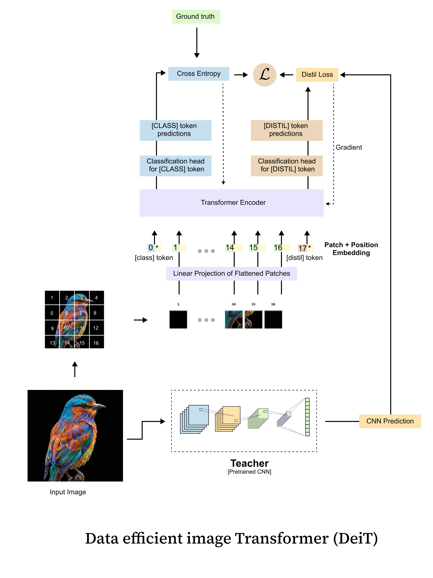
Figure 1.7 The DeiT architecture extends the standard Vision Transformer with a distillation token. The input image is divided into fixed-size patches, which are linearly projected into embeddings. Two special tokens are prepended: the [CLS] token (supervised by ground-truth labels) and the [DIST] token (supervised by the teacher model's predictions). Both tokens pass through all transformer encoder layers, interacting with patch tokens and with each other through self-attention. At the output, separate classification heads produce predictions from each token.
The architecture works as follows:
Patch embedding. The input image (e.g., 224x224 pixels) is divided into non-overlapping patches (e.g., 16x16 pixels each), yielding a sequence of
\(N = (224/16)^2=196 \)patches. Each patch is linearly projected into a D-dimensional embedding vector using a learnable projection matrix. In practice, this is implemented as a single convolution with kernel size and stride equal to the patch size.
Special tokens. Two learnable embedding vectors are prepended to the sequence:
The [CLS] token: a standard classification token (as in the original ViT) that aggregates information for predicting the ground-truth label.
The [DIST] token: a novel distillation token that aggregates information for mimicking the teacher model’s predictions.
Positional embeddings. Learnable 1D position embeddings are added to all tokens (patches + CLS + DIST), giving the model information about spatial arrangement. The total sequence length is N+2.
Transformer encoder. The sequence passes through L standard transformer encoder layers, each consisting of multi-head self-attention (MSA) and a feed-forward network (FFN). Both special tokens interact with all patch tokens and with each other through self-attention.
Dual classification heads. At the output, two separate linear heads produce predictions:
\(\mathbf{z}_{s}^{\text{cls}} = W_{\text{cls}} \cdot \mathbf{x}_{\text{cls}}\)\(\text{logits from the CLS token, trained against ground-truth labels.}\)\(\mathbf{z}_{s}^{\text{dist}} = W_{\text{dist}} \cdot \mathbf{x}_{\text{dist}}\)\(\text{ logits from the DIST token, trained against the teacher's predictions.}\)Inference. At test time, the predictions from both heads are combined by averaging the softmax outputs:
\(\mathbf{p}_{\text{inference}} = \frac{1}{2}\left[\sigma(\mathbf{z}_s^{\text{cls}}) + \sigma(\mathbf{z}_s^{\text{dist}})\right] \)
Now let us look at the original architecture diagram from the paper for additional perspective.
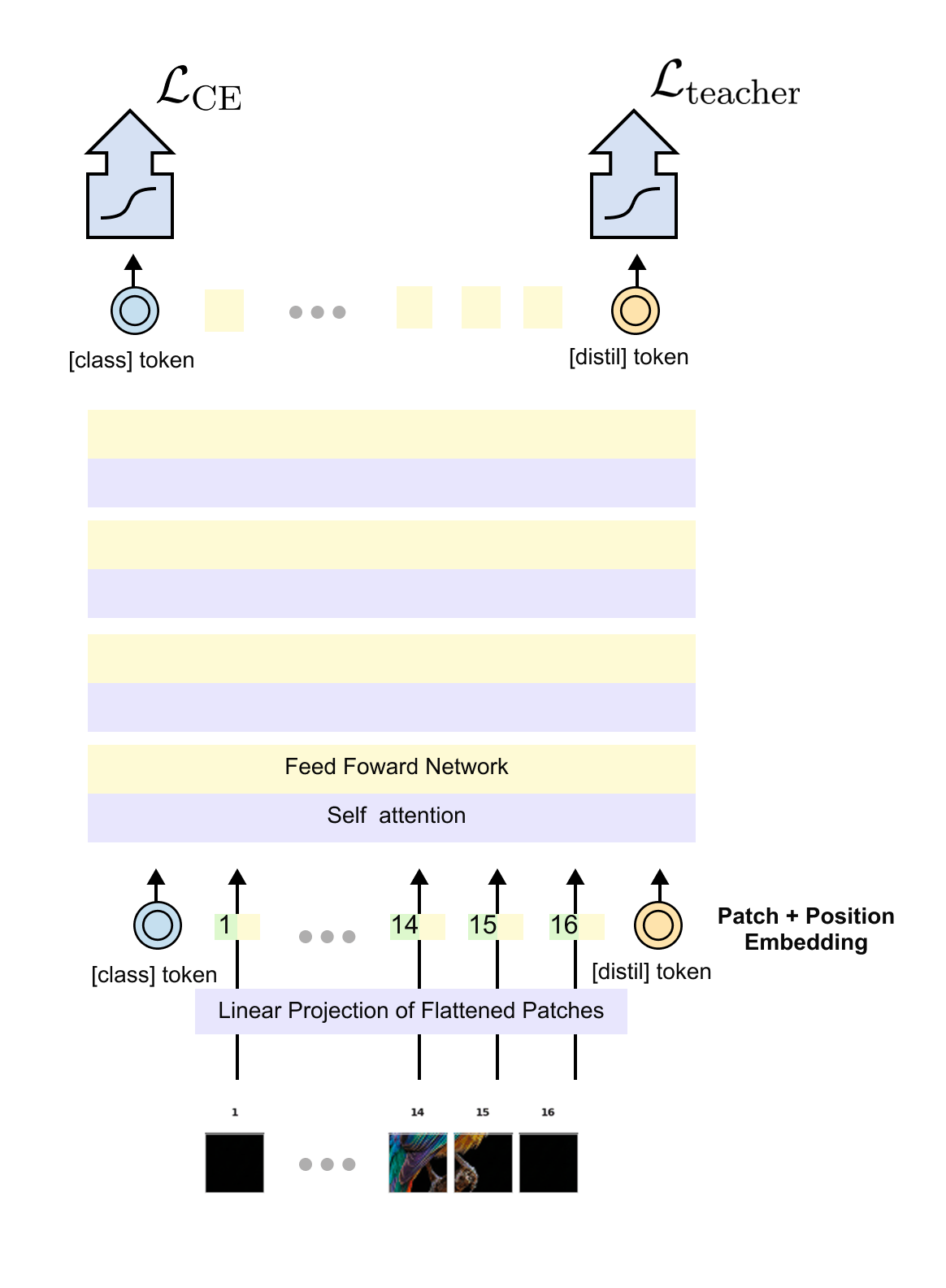
Figure 1.8 The DeiT architecture as presented in the original paper, showing the complete training pipeline. The student (Vision Transformer) receives supervision from two sources: the ground-truth labels (via cross-entropy on the CLS token) and the pre-trained CNN teacher (via the distillation loss on the DIST token). The teacher model is frozen during training and its weights are never updated. The distillation token enables the transformer to learn the CNN's implicit understanding of image structure without architecturally constraining itself.
Why a separate distillation token?
You might wonder: why not simply add the teacher’s loss to the existing CLS token? Why introduce a separate token? The DeiT paper provides a compelling empirical answer.
The authors experimented with using two identical CLS tokens (both trained on ground-truth labels) and found that they converge to nearly identical representations, with cosine similarity approaching 0.999. They carry redundant information.
In contrast, the CLS token and distillation token, trained on different objectives, develop meaningfully different representations. Their cosine similarity is approximately 0.06 in early layers and rises to only about 0.93 by the final layer. This means the distillation token captures complementary information that the CLS token alone would miss. The two tokens learn different “perspectives” on the input, and combining them at inference yields better predictions than either alone.
The teacher model
DeiT uses a pre-trained CNN as the teacher. In the paper, the primary teacher is RegNetY-16GF (84 million parameters, 82.9% top-1 accuracy on ImageNet), though the authors also experimented with other architectures. Critically, the teacher is frozen during training: its weights are never updated. It simply provides predictions that the student learns to mimic.
A surprising finding from the paper is that a CNN teacher produces dramatically better student performance than a transformer teacher. The authors note that the transformer student “learned least from a transformer-teacher but learned most from a big convolution-teacher.” This supports the hypothesis that distillation effectively transfers the CNN’s inductive biases (locality, translation equivariance) to the transformer student, giving it the benefits of both architectures.
But how exactly does knowledge transfer from teacher to student? To understand this, we need to dive deep into the mechanics of knowledge distillation.
1.4 Knowledge distillation: teaching a student network
Knowledge distillation is a model compression technique where a small student model is trained to mimic the behavior of a larger, more capable teacher model. The goal is to produce a compact model that retains much of the teacher’s performance while being faster and cheaper at inference. Let us trace the evolution of this idea and then build up the mathematics step by step.
A brief history
The idea of compressing knowledge from large models into small ones dates back to 2006, when researchers at Cornell University proposed model compression. At the time, the best-performing models were not single networks but ensembles of hundreds or thousands of models whose predictions were averaged. These ensembles were accurate but far too large for deployment on devices like PDAs (personal digital assistants, the predecessors to smartphones).
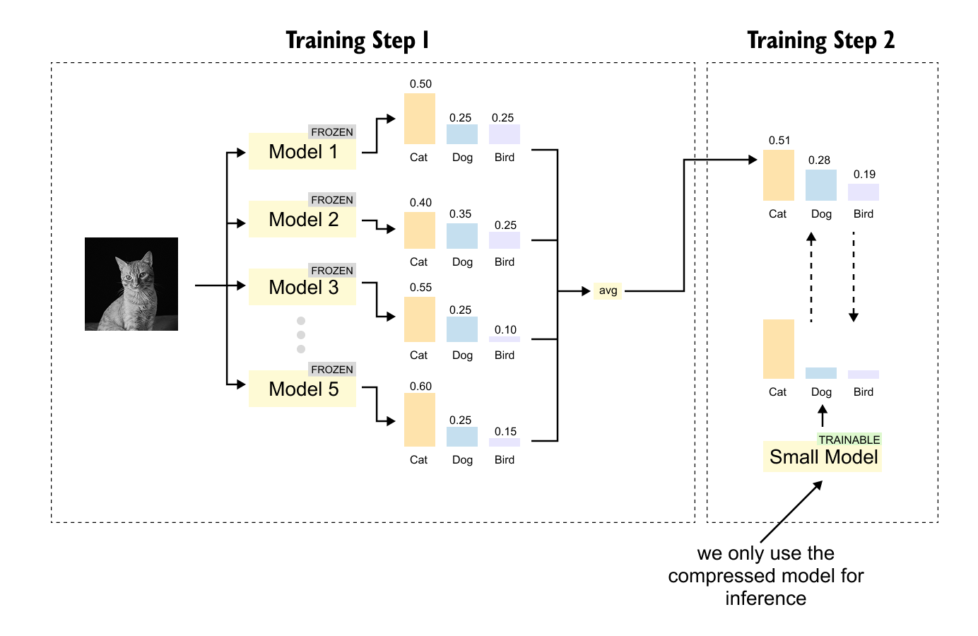
Figure 1.9 The two-step process of model compression, as introduced in 2006. In Step 1, an ensemble of multiple models is trained, with each model making independent predictions. In Step 2, a single small model is trained to directly predict the averaged output of the ensemble, compressing the knowledge of many models into one.
The insight was elegantly simple: instead of shipping all the ensemble models to the device, train a single small model to predict the ensemble's averaged output. This small model captures the collective wisdom of the ensemble while being compact enough for deployment.
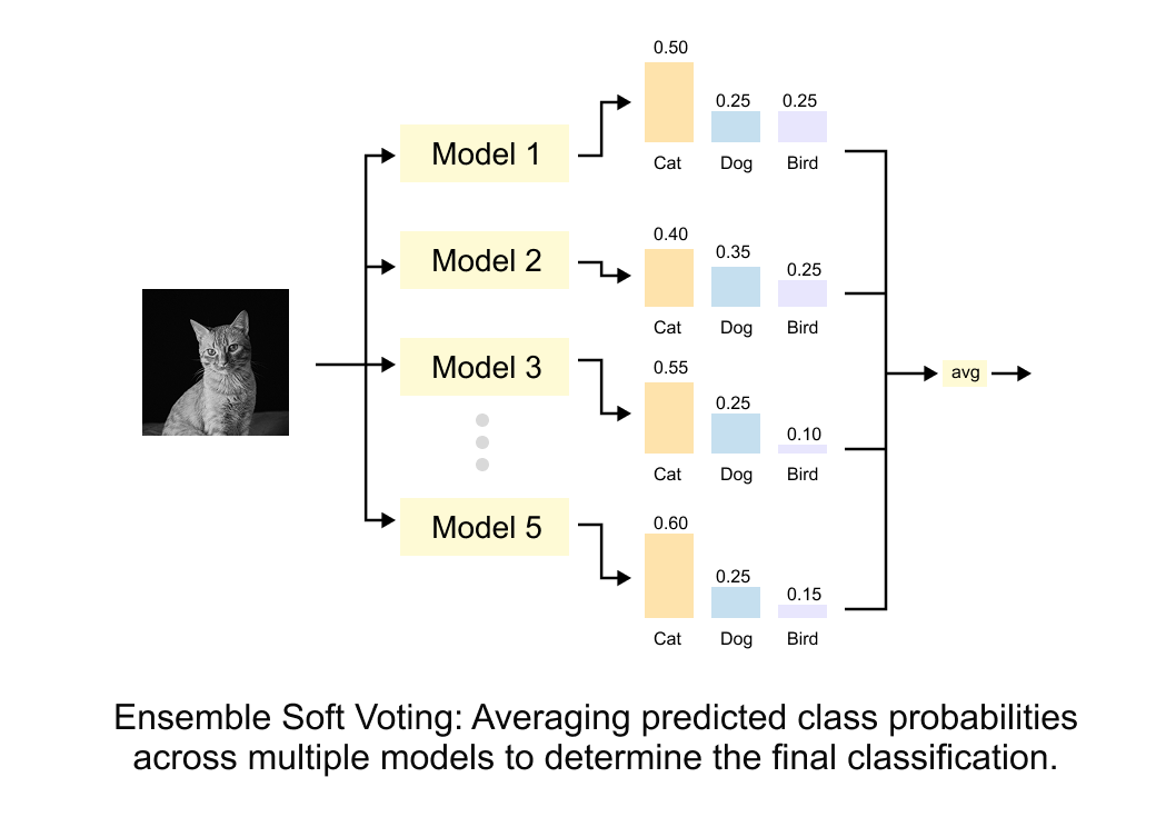
Figure 1.10 Ensemble soft voting. Multiple models (Model 1 through Model 5) each output a probability distribution over classes. These distributions are averaged to produce a final classification. The key insight is that this averaged distribution carries more information than any single model’s hard prediction.
In 2015, Geoffrey Hinton and Jeff Dean (at Google) revisited this idea and gave it the name we use today: knowledge distillation. Their crucial insight was that distillation is valuable even without an ensemble. A single large model’s soft probability outputs carry richer information than hard labels alone, and this information can be transferred to a smaller student.
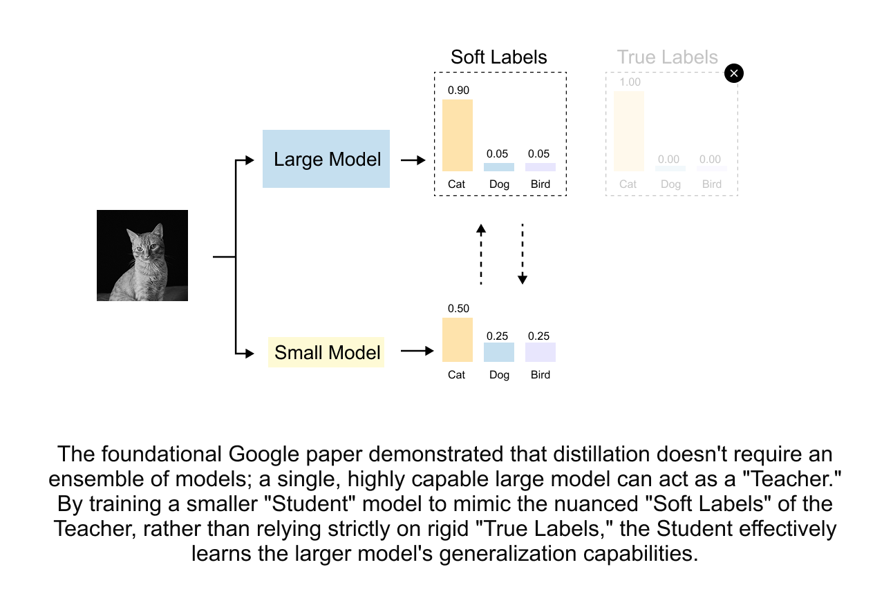
Figure 1.11 Knowledge distillation does not require an ensemble. A single large teacher model generates soft labels (probability distributions) that carry more information than one-hot hard labels. The student learns from these enriched targets, inheriting the teacher’s nuanced understanding of inter-class relationships.
Hard labels vs. soft labels: the concept of dark knowledge
To understand why soft labels are so valuable, consider a concrete example. Suppose we have a teacher model classifying animal images into three categories: dog, cat, and mouse.
Given an image of a husky, the hard label (ground truth) is simply:
This tells the student: "This is a dog. Period." But the teacher's soft prediction might be:
This soft distribution tells the student something much richer: “This is most likely a dog, but it looks somewhat like a cat (perhaps because of the fur texture), and it looks very little like a mouse.” This additional information about what the input is not (and how much it is “not” each class) is what Hinton poetically called dark knowledge.

Figure 1.12 Dark knowledge revealed through soft labels. While hard labels simply say "this is a husky," the teacher's soft probability distribution reveals richer inter-class relationships. A husky image gets high probability for "husky" but also notable probability for "wolf" and some for "dog," reflecting visual similarities between these animals that the teacher has learned. This relational information (the dark knowledge) helps the student learn more efficiently.
Dark knowledge encodes the teacher’s learned understanding of inter-class similarities and relationships. A husky looks more like a wolf than like a goldfish. A handwritten “7” looks more like a “1” than like a “0.” These relational insights are completely absent from one-hot hard labels but are naturally present in soft probability distributions.
The mathematics of knowledge distillation
Now let us formalize the distillation process mathematically. The framework involves three key components: temperature scaling, the distillation loss function, and the combined training objective.
Temperature scaling
When a well-trained teacher model makes predictions, its output distribution is often very “peaked”: the correct class gets probability close to 1.0, and all other classes get near-zero probabilities. For example:
These near-zero probabilities contain the dark knowledge we want to transfer, but they are so small that they provide almost no gradient signal during training. The student cannot learn from values like 0.005 because the gradients are essentially zero.
Temperature scaling solves this by softening the probability distribution. Given a vector of logits
(the raw, unnormalized outputs of the network before softmax), the standard softmax function is:
With a temperature parameter τ>0 , we define the temperature-scaled softmax:
The temperature controls how "spread out" the distribution is:
Standard softmax. The distribution reflects the model's learned confidence.
Higher temperature softens the distribution, making all probabilities more uniform and revealing the relative differences between logits. This amplifies dark knowledge.
The distribution approaches a uniform distribution 1/K for K classes.
The distribution collapses to a one-hot vector concentrated on the largest logit (argmax).
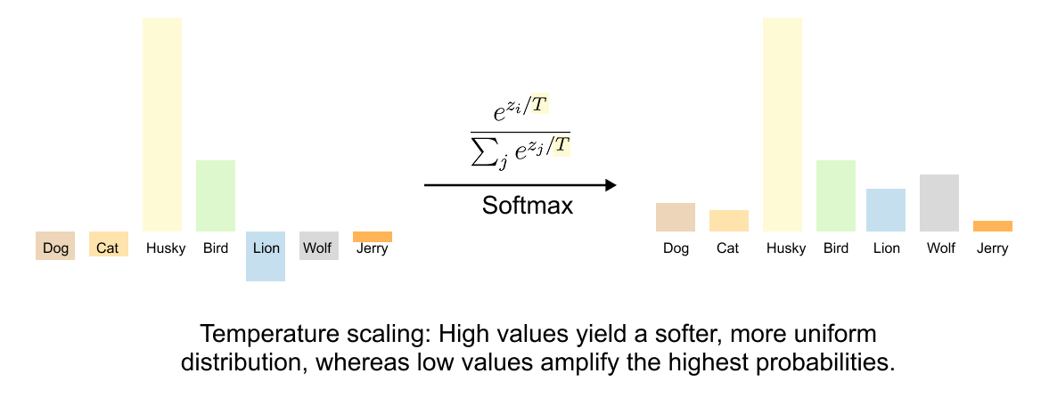
Figure 1.13 The effect of temperature on softmax distributions. The formula shows how temperature controls the “peakiness” of the output. Left: the raw logit values before temperature-scaled softmax. Right: after applying softmax with high temperature, the distribution becomes more uniform, revealing the relative magnitudes of all logits. This smoothing is essential for transferring dark knowledge from teacher to student.
Let us work through a concrete numerical example. Suppose a teacher produces logits z=[5.0,2.0,1.0] for three classes. Here is how temperature affects the resulting probabilities:
At τ=1, the distribution is peaked: dog gets 93.6% and the dark knowledge (cat and mouse probabilities) is barely visible. At τ=5, the distribution is much flatter: we can clearly see that the teacher considers this image more cat-like than mouse-like (27.5% vs. 22.5%). This relational information is the dark knowledge that distillation transfers.
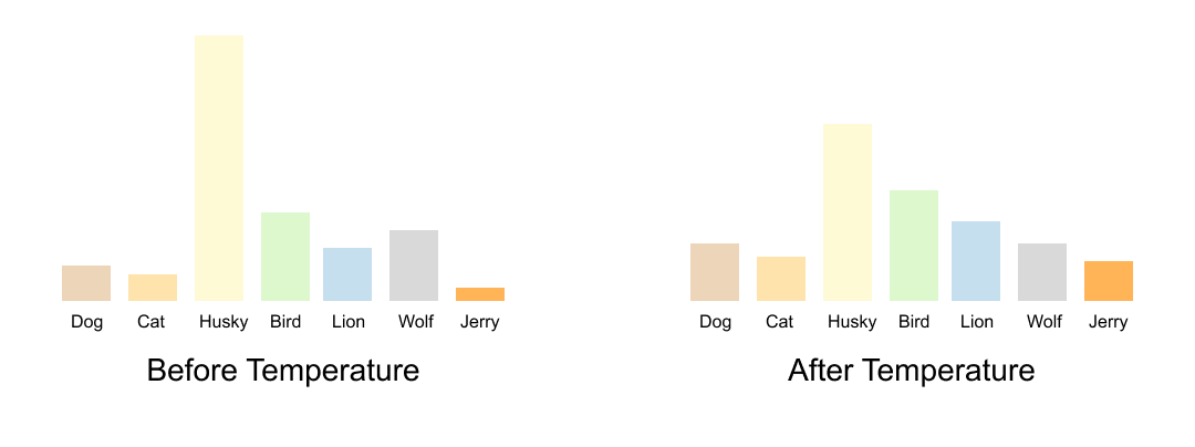
Figure 1.14 A direct comparison of probability distributions before and after temperature scaling. The left distribution (low temperature) shows sharp peaks where the correct class dominates. The right distribution (high temperature) shows a smoothed version where the relative probabilities of non-dominant classes become visible. This smoothing allows the student to learn not just which class is correct, but which incorrect classes are most similar to the correct one.
Cross-entropy loss
The standard classification loss in deep learning is cross-entropy. For a ground-truth one-hot label y=[y1,y2,…,yK] and predicted probabilities p=[p1,p2,…,pK], the cross-entropy is:
Since y is one-hot with y_c=1 for the true class cc and y_i=0 for all other classes, this simplifies to:
Let us verify with an example. If the true class is "cat" (c=1) and the model predicts p=[0.80,0.15,0.05]:
A confident correct prediction gives a low loss. If instead pc=0.1:
An incorrect or uncertain prediction gives a high loss, pushing the model to adjust its weights. Note that −log(x) produces a positive value when x∈(0,1), which is always the case for probabilities.
KL divergence
While cross-entropy measures how well predictions match a target distribution, Kullback-Leibler (KL) divergence measures how different two probability distributions are from each other. For distributions p (teacher) and q (student):
KL divergence has several important properties:

Let us work through a concrete example. Suppose the teacher outputs
and the student outputs
A small KL divergence indicates the student is already quite close to the teacher. Now consider an overconfident student that outputs
The KL divergence is larger because the student is more confident than the teacher. KL divergence heavily penalizes cases where the student assigns very low probability to classes that the teacher considers plausible.
NOTE
There is an important mathematical subtlety about KL divergence when pi=0. Since
\(\lim_{x \to 0^+} x \log(x) = 0\)(which can be verified using L'Hôpital's rule), terms where pi=0 contribute zero to the divergence. This means the KL divergence is well-defined even when the teacher assigns zero probability to some classes.
The relationship between KL divergence and cross-entropy is:
where
is the cross-entropy and
is the entropy of the teacher distribution. Since the teacher is frozen, H(p) is a constant, and minimizing KL divergence is equivalent to minimizing the cross-entropy between teacher and student distributions.
The complete knowledge distillation loss
Putting it all together, the knowledge distillation loss from Hinton et al. (2015) combines two terms:

The first term is the standard cross-entropy between the student’s predictions (at τ=1) and the ground-truth labels. This keeps the student honest: it must still learn to classify correctly.
The second term is the KL divergence between the teacher’s and student’s softened predictions (both at temperature τ). This transfers the dark knowledge from teacher to student.
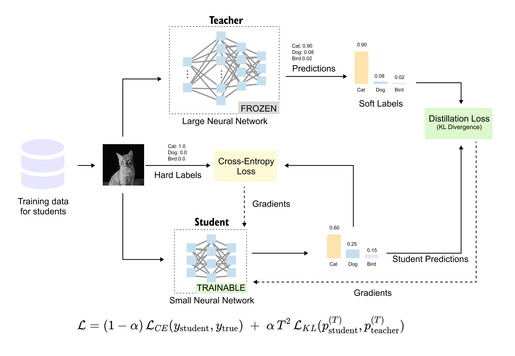
Figure 1.15 The complete knowledge distillation framework. Training data feeds into both the teacher (large network, frozen) and the student (small network, being trained). The teacher produces soft labels via temperature-scaled softmax, while the ground truth provides hard labels. The student's total loss combines two components: the cross-entropy loss L_CE against hard labels, and the KL divergence loss L_KL against the teacher's soft labels. The formula
weights these components, and gradients flow back through the student to update its weights.
You may wonder why the KL divergence term is multiplied by τ^2. This is not arbitrary; it is a mathematical necessity for keeping the gradient magnitudes balanced.
When we compute the gradient of the soft cross-entropy loss with respect to the student's logits zs,i:
The temperature scaling introduces a factor of 1/τ in the gradient. Additionally, the softened probabilities themselves compress the differences between logits by another factor of approximately 1/τ, yielding an overall gradient scaling of approximately 1/τ2.
Without compensation, the soft-label gradients would vanish as we increase temperature, defeating the purpose of softening. The τ_2 multiplier restores the gradient magnitudes to be comparable with the hard-label loss, ensuring that the weighting coefficient αα behaves predictably regardless of the chosen temperature.
High-temperature approximation: why distillation equals logit matching
There is an elegant mathematical insight that connects distillation to a simpler concept. At high temperatures, the softmax can be approximated using a Taylor expansion:
where
is the mean logit and K is the number of classes.
Substituting this into the KL divergence and simplifying, the soft-label loss reduces to:
This is simply a mean squared error between the logits of the student and teacher! At high temperature, knowledge distillation is approximately equivalent to logit matching, which was actually proposed in 2014 as a precursor to Hinton's method. The τ_2 factor cancels the 1/τ2 scaling, confirming that the multiplication is necessary. This result also reveals why dark knowledge transfer works: the student is effectively learning the teacher's internal ranking of all classes, not just its top prediction.
1.5 DeiT’s distillation: hard labels beat soft labels
Now that we understand the mechanics of knowledge distillation, let us see how DeiT adapts this framework. DeiT introduces two variants: soft distillation and hard distillation. Surprisingly, the simpler approach wins.
Soft distillation in DeiT
DeiT’s soft distillation uses the standard knowledge distillation framework, but with the distillation token producing separate logits:

The CLS token head learns from ground-truth labels. The distillation token head learns to match the teacher’s full soft probability distribution.
Hard distillation in DeiT
Hard distillation replaces the KL divergence with a simple cross-entropy against the teacher’s hard prediction (argmax):
This is remarkably simple: no temperature parameter, no KL divergence, no τ2 correction. Just two cross-entropy losses weighted equally. The CLS token learns from the ground truth, and the distillation token learns from the teacher’s top-1 prediction.
Why hard distillation works better
The DeiT paper found that hard distillation outperforms soft distillation by approximately +1.0--1.2% accuracy on ImageNet. This was surprising because soft labels contain strictly more information than hard labels.
The authors hypothesize that this relates to the fundamental difference between the teacher (a CNN) and the student (a transformer). CNNs and transformers process visual features in fundamentally different ways: CNNs use local convolutional filters while transformers use global self-attention. When the teacher provides a full soft distribution, it reflects the CNN’s specific way of processing the image, which may not transfer well to the transformer’s very different processing pipeline. Hard labels abstract away these architectural details, providing a cleaner supervisory signal that is easier for the transformer to learn from.
Think of it like learning to cook. Soft distillation is like watching a master chef’s exact hand movements (which depend on their specific knife and grip style). Hard distillation is like reading their recipe (the end result, abstracted from the specific process). If you have different tools and a different grip, the recipe is more useful than mimicking movements that do not suit your tools.
DeiT results
The results are compelling. Figure 1.16 shows the performance-throughput trade-off for various models.
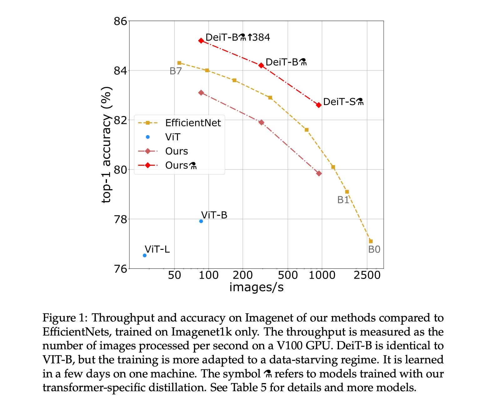
Figure 1.16 Performance comparison between DeiT variants and competing architectures, plotting throughput (images per second, higher is better) against ImageNet top-1 accuracy (higher is better). DeiT-B with distillation (marked with the alembic symbol) achieves 85.2% accuracy, matching or exceeding EfficientNet while being significantly faster at inference. The key takeaway is that DeiT achieves competitive accuracy with ViT-level throughput, using only ImageNet-1K for training rather than the 300 million images that the original ViT required.
DeiT demonstrated that the Vision Transformer’s dependence on massive datasets was not an inherent limitation of the architecture, but a training problem with a training solution. By combining knowledge distillation with a dedicated distillation token, DeiT gave the transformer a way to absorb the inductive biases of a CNN teacher without modifying the transformer architecture itself. The CLS token learns from ground truth labels while the distillation token learns from the teacher’s predictions, and the two complementary signals together produce a model that generalizes better than either supervision source alone. This insight, that architectural inductive biases can be transferred rather than engineered, opened the door to practical vision transformers that anyone with a single multi-GPU machine could train.
1.6 Building DeiT from scratch in PyTorch
Data Efficient Image Transformer Code is available below
https://github.com/VizuaraAI/Transformers-for-vision-BOOK
[Don’t forget to star the code repo!]
With the theory firmly established, let us now build a complete DeiT implementation from scratch. We will train a small-scale version on MNIST digits to demonstrate all the key concepts: patch embedding, the distillation token, the teacher-student setup, and the knowledge distillation loss. While MNIST is far simpler than ImageNet, it lets us see the entire pipeline working end-to-end on a single machine.
Setting up imports and configuration
We begin by importing the necessary libraries and defining our hyperparameters. We will use PyTorch for the implementation, torchvision for datasets and the pre-trained teacher model, and NumPy for utility operations.
Listing 1.1 Importing libraries and setting up the device
import torch
import torch.nn as nn
import torch.nn.functional as F
import torchvision
from torch.utils.data import Subset, DataLoader
from torchvision import transforms, datasets, models
import numpy as np
import matplotlib.pyplot as plt

device = 'cuda' if torch.cuda.is_available() else 'cpu' #A
#A Automatically selects GPU if available, otherwise falls back to CPU
Next, we define the hyperparameters that control our model and training process. These values are deliberately small compared to the full DeiT paper to allow rapid experimentation on a personal machine.
Listing 1.2 Defining hyperparameters
BATCH_SIZE = 12
ATTENTION_HEADS = 4          #A
TRANSFORMER_LAYERS = 4       #B
EMBED_DIM = 16               #C
IMG_SIZE = 28                #D
PATCH_SIZE = 7               #E
CLASSES = 10                 #F
EPOCHS_STUDENT = 10
LR_STUDENT = 1e-4
TEMPERATURE = 4              #G
ALPHA = 0.1                  #H
CHANNELS = 3                 #I
#A Number of attention heads in each transformer layer
#B Number of stacked transformer encoder layers
#C Embedding dimension for patch tokens (small for demonstration)
#D MNIST images are 28x28 pixels
#E Each patch is 7x7 pixels, giving us (28/7)^2 = 16 patches
#F MNIST has 10 digit classes (0--9)
#G Temperature for softening the teacher's probability distribution
#H Weight for the KL divergence term in the distillation loss
#I Number of input channels (expanded from 1 to 3 for CNN compatibility)
Let us understand the patch arithmetic. With 28x28 images and 7x7 patches, each image is divided into
non-overlapping patches. Each patch is flattened and linearly projected into a 16-dimensional embedding. Together with the CLS token and distillation token, this gives us a sequence of 16+2=18 tokens.
Preparing the data
MNIST images are grayscale (1 channel), but our teacher model (ResNet50) expects 3-channel RGB inputs. We handle this by repeating the single channel three times. We also use only 10% of the training set to simulate a data-scarce scenario, which is the exact setting where DeiT’s distillation approach shines.
Listing 1.3 Loading and preparing the MNIST dataset
tfm = transforms.Compose([
    transforms.ToTensor(),
    transforms.Lambda(lambda t: t.repeat(3, 1, 1)),    #A
])

train_full = datasets.MNIST('./data', train=True, download=True, transform=tfm)
test = datasets.MNIST('./data', train=False, download=True, transform=tfm)

n = int(0.1 * len(train_full))                         #B
subset_idx = np.random.permutation(len(train_full))[:n]
train = Subset(train_full, subset_idx)

train_dl = DataLoader(train, batch_size=BATCH_SIZE, shuffle=True)
test_dl = DataLoader(test, batch_size=BATCH_SIZE)
#A Converts single-channel grayscale to 3-channel by repeating, making it compatible with the ResNet teacher
#B Uses only 10% of training data (6,000 images from 60,000) to simulate data scarcity
Using only 6,000 training images is deliberately challenging. This mimics the real-world scenario that motivated DeiT: how do we train a Vision Transformer effectively when data is limited? Knowledge distillation is the answer.
Setting up the teacher model
Our teacher is a pre-trained ResNet50, one of the most well-known CNN architectures. We load it with ImageNet pre-trained weights and modify the final classification layer to output 10 classes (for MNIST digits) instead of the original 1,000 ImageNet classes.
Critically, we freeze all the teacher’s parameters except the final classification layer. The teacher’s convolutional feature extractors already understand visual patterns from ImageNet pre-training. We only need to adapt the final layer to map those features to our 10 digit classes.
Listing 1.4 Setting up the pre-trained CNN teacher
teacher = models.resnet50(weights=models.ResNet50_Weights.IMAGENET1K_V2)
teacher.fc = nn.Linear(teacher.fc.in_features, CLASSES)    #A
teacher.to(device)

for param in teacher.parameters():                         #B
    param.requires_grad = False

for param in teacher.fc.parameters():                      #C
    param.requires_grad = True
#A Replaces the 1000-class ImageNet head with a 10-class head for MNIST
#B Freezes all layers: the convolutional backbone will not be updated
#C Unfreezes only the final classification layer so it can learn MNIST-specific mappings
This setup mirrors the DeiT paper’s approach: the teacher is a powerful CNN that has already learned rich visual representations. By freezing its backbone, we preserve the inductive biases (locality, translation equivariance, hierarchical features) that the CNN learned during ImageNet pre-training. The student will learn to mimic these capabilities through distillation.
Building the student Vision Transformer
Now we build the student model: a Vision Transformer with a distillation token. This is the heart of the DeiT architecture. Let us break it into two components: the patch embedding layer and the full ViT model.
Listing 1.5 Patch embedding module
class PatchEmbed(nn.Module):
    def __init__(self, img_size=IMG_SIZE, patch=PATCH_SIZE,
                 dim=EMBED_DIM, channels=CHANNELS):
        super().__init__()
        self.proj = nn.Conv2d(channels, dim, patch, patch)  #A
        self.n = (img_size // patch) ** 2                   #B

    def forward(self, x):
        x = self.proj(x)           #C
        x = x.flatten(2)           #D
        x = x.transpose(1, 2)     #E
        return x
#A A Conv2d with kernel_size=patch_size and stride=patch_size extracts non-overlapping patches and projects them to the embedding dimension in one operation
#B Computes the number of patches: (28/7)^2 = 16 patches
#C Applies the convolution: (B, 3, 28, 28) -> (B, 16, 4, 4)
#D Flattens the spatial dimensions: (B, 16, 4, 4) -> (B, 16, 16)
#E Transposes to get sequence format: (B, 16, 16) -> (B, 16, 16) where first 16 is sequence length and second 16 is embedding dim
The patch embedding uses a single convolution to simultaneously extract patches and project them into the embedding space. This is mathematically equivalent to extracting each patch, flattening it, and multiplying by a weight matrix, but it is computationally more efficient.
Now let us build the full ViT model with the distillation token:
Listing 1.6 The DeiT student model with distillation token
class ViT(nn.Module):
    def __init__(self, num_classes=CLASSES, dim=EMBED_DIM,
                 depth=TRANSFORMER_LAYERS, heads=ATTENTION_HEADS):
        super().__init__()
        self.patch = PatchEmbed()
        n = self.patch.n

        self.cls = nn.Parameter(torch.zeros(1, 1, dim))      #A
        self.distill = nn.Parameter(torch.zeros(1, 1, dim))   #B
        self.pos = nn.Parameter(torch.zeros(1, n + 2, dim))   #C

        self.blocks = nn.Sequential(*[                        #D
            nn.TransformerEncoderLayer(
                dim, heads, dim * 4, batch_first=True
            )
            for _ in range(depth)
        ])

        self.norm = nn.LayerNorm(dim)                         #E
        self.head_cls = nn.Linear(dim, num_classes)           #F
        self.head_dist = nn.Linear(dim, num_classes)          #G

    def forward(self, x):
        B = x.size(0)
        x = self.patch(x)                                     #H

        cls = self.cls.expand(B, -1, -1)                      #I
        dist = self.distill.expand(B, -1, -1)

        x = torch.cat([cls, x, dist], dim=1) + self.pos      #J

        x = self.blocks(x)                                    #K
        x = self.norm(x)

        cls_out = x[:, 0]                                     #L
        dist_out = x[:, -1]                                   #M

        cls_logits = self.head_cls(cls_out)                    #N
        dist_logits = self.head_dist(dist_out)

        return cls_logits, dist_logits

student = ViT().to(device)
opt_s = torch.optim.AdamW(student.parameters(), lr=LR_STUDENT)
#A Learnable CLS token: initialized to zeros, shape (1, 1, dim)
#B Learnable distillation token: the key DeiT innovation, also initialized to zeros
#C Positional embeddings for all tokens: n patches + CLS + DIST = 18 positions
#D Stack of transformer encoder layers, each with multi-head self-attention and FFN
#E Layer normalization applied after the final transformer block
#F Classification head for the CLS token (trained against ground truth)
#G Separate classification head for the distillation token (trained against teacher)
#H Convert image to patch embeddings: (B, 3, 28, 28) -> (B, 16, 16)
#I Expand special tokens to match batch size: (1, 1, 16) -> (B, 1, 16)
#J Concatenate CLS + patches + DIST and add positional embeddings: (B, 18, 16)
#K Pass through all transformer encoder layers
#L Extract the CLS token output (first position)
#M Extract the distillation token output (last position)
#N Produce class logits from each token through separate linear heads
There are several important details to notice in this implementation:
Two separate learnable tokens. Both
self.clsandself.distillarenn.Parameterobjects initialized to zeros. During training, backpropagation will update them to learn useful representations. Despite identical initialization, they will diverge because they receive different gradient signals (ground-truth loss vs. teacher loss).Positional embeddings. The
self.postensor has shape(1, n+2, dim), providing a unique positional encoding for each of the 18 positions. This is essential because, unlike CNNs, the transformer has no built-in notion of spatial arrangement.Two output heads. The
head_clsandhead_distare separate linear layers that map the final token representations to class logits. Each head receives its own supervision signal during training.Token placement. The CLS token is placed at position 0 and the distillation token at the last position. This is a convention; both tokens interact with all patch tokens through self-attention regardless of their position.
Implementing the knowledge distillation loss
Now we implement the loss function that drives the distillation process. This is where the mathematics we developed earlier becomes code.
Listing 1.7 Knowledge distillation loss function
def kd_loss(s_logits, t_logits, y, T=TEMPERATURE, alpha=ALPHA):
    kd = F.kl_div(                                        #A
        F.softmax(s_logits / T, dim=1),                   #B
        F.softmax(t_logits / T, dim=1),                   #C
        reduction='batchmean'
    ) * (T * T)                                           #D
    ce = F.cross_entropy(s_logits, y)                     #E
    return alpha * kd + (1 - alpha) * ce                  #F
#A KL divergence between the student’s and teacher’s softened distributions #B Student’s log-probabilities at temperature T (PyTorch’s kl_div expects log-probabilities for the first argument)
#C Teacher’s probabilities at temperature T (target distribution)
#D Multiply by T^2 to compensate for the reduced gradient magnitude
#E Standard cross-entropy between student predictions and ground-truth labels
#F Weighted combination: alpha controls the distillation-vs-classification balance
Let us trace through this function to make sure we understand each step. Given student logits z_s, teacher logits z_t, ground-truth labels y, temperature T=4, and α=0.1:
F.softmax(s_logits / T, dim=1)computes σ(zs/4): the student’s softened probabilitiesF.softmax(t_logits / T, dim=1)computes σ(zt/4): the teacher’s softened probabilitiesF.kl_div(...)computes D_KL(teacher∥student), the divergence between these distributionsMultiplying by T^2=16 compensates for the gradient scaling
F.cross_entropy(s_logits, y)computes L_CE at τ=1The final loss is 0.1×(KL term)+0.9×(CE term)
With α=0.1, we weight the cross-entropy heavily (90%) and the distillation lightly (10%). This means the student primarily learns from the ground-truth labels, with the teacher’s knowledge providing supplementary guidance.
Training the student
With all components in place, we can now train the student model. The training loop follows the standard PyTorch pattern, but with the crucial addition of generating teacher predictions on the fly.
Listing 1.8 Training the DeiT student with knowledge distillation
print("Training student...")
for e in range(EPOCHS_STUDENT):
    student.train()
    for x, y in train_dl:
        x, y = x.to(device), y.to(device)

        with torch.no_grad():                            #A
            t_logits = teacher(x)

        cls_logits, dist_logits = student(x)             #B
        loss_cls = F.cross_entropy(cls_logits, y)

        loss_distill = kd_loss(dist_logits, t_logits, y) #C
        loss = loss_distill + loss_cls
        opt_s.zero_grad()                                #D
        loss.backward()
        opt_s.step()

    print(f"Epoch {e+1} done")
Output
Training student...
Epoch 1 done
Epoch 2 done
Epoch 3 done
Epoch 4 done
Epoch 5 done
Epoch 6 done
Epoch 7 done
Epoch 8 done
Epoch 9 done
Epoch 10 done
#A Teacher inference with no gradient tracking: the teacher is frozen and never updated
#B Student forward pass returns two sets of logits (CLS and distillation)
#C CLS loss trains the classification head with hard labels; distillation loss aligns the DIST token's logits with the teacher's soft logits. The total loss combines both.
#D Standard gradient descent: zero gradients, compute backpropagation, update weights
There is an important detail to highlight: we pass dist_logits (from the distillation token) to the loss function, not cls_logits. The distillation token is specifically designed to learn from the teacher. In a full DeiT implementation, you would compute a separate cross-entropy loss for the CLS token against ground truth and add it to the distillation loss. In our simplified version, the kd_loss function handles both terms using the distillation token.
Notice the torch.no_grad() context manager around the teacher’s forward pass. Since the teacher is frozen, we do not need to track gradients for its computations. This saves memory and computation: we only backpropagate through the student.
Evaluating the trained model
After training, we evaluate the student by combining the predictions from both tokens. At inference time, the CLS and distillation tokens each produce their own logits, and we average the softmax outputs to get the final prediction.
Listing 1.9 Evaluating the DeiT student
student.eval()
correct = 0
total = 0
samples = []

with torch.no_grad():                                     #A
    for x, y in test_dl:
        x, y = x.to(device), y.to(device)
        cls_logits, dist_logits = student(x)

        cls_dist = (cls_logits + dist_logits) / 2          #B
        pred = cls_dist.argmax(1)                          #C

        correct += (pred == y).sum().item()
        total += y.size(0)

        if len(samples) < 15:
            samples.append((x.cpu(), pred.cpu(), y.cpu()))

acc = 100 * correct / total
print(f"Test Accuracy: {acc:.2f}%")
#A No gradient computation needed during evaluation
#B Average the logits from both tokens: this combines the ground-truth-informed CLS prediction with the teacher-informed distillation prediction
#C Take the class with highest average logit as the final prediction
The averaging of CLS and distillation logits at inference is a key DeiT design choice. Each token has learned a different perspective on the input: the CLS token is optimized for ground-truth classification, while the distillation token is optimized for mimicking the teacher. Combining them yields a prediction that benefits from both information sources.
Finally, we can visualize some predictions to qualitatively assess the model:
Listing 1.10 Displaying sample predictions
fig, axs = plt.subplots(1, len(samples), figsize=(12, 3))
for i, (img, pred, true) in enumerate(samples):
    img = img[0].permute(1, 2, 0).numpy()                 #A
    axs[i].imshow(img)
    axs[i].set_title(f"P:{pred[0].item()} T:{true[0].item()}")  #B
    axs[i].axis('off')
plt.show()
Output

#A Convert from (C, H, W) tensor format to (H, W, C) NumPy array for matplotlib
#B Display the predicted label (P) and true label (T) for each sample
With this minimal implementation, we achieve approximately 94% accuracy on MNIST using only 6,000 training images and 100 epochs in just 18 mins of training on T4 GPU. While this is modest compared to state-of-the-art results, remember that we are using an extremely small model (16-dimensional embeddings, 4 layers, 4 heads) with very little data and training time. On the full ImageNet dataset with the proper hyperparameters from section 1.5, DeiT-B achieves 83.4% top-1 accuracy, competitive with models trained on 250 times more data.
The code demonstrates all the core DeiT concepts:
Patch embedding via convolution
CLS and distillation tokens as learnable parameters
Dual classification heads with separate objectives
Knowledge distillation loss combining cross-entropy and KL divergence
Temperature scaling for softening probability distributions
Averaging token predictions at inference
Summary
Inductive biases are built-in architectural assumptions that shape how a model learns. CNNs have strong inductive biases (locality and translation equivariance) that make them data-efficient but limit their ability to capture long-range dependencies
Vision Transformers lack these biases, processing all patches globally through self-attention. This flexibility becomes an advantage with enough data (300 million images) but a severe limitation with standard datasets (1.2 million images), causing overfitting and poor generalization
Scaling laws show that model performance follows predictable power-law relationships with model size, dataset size, and compute. These laws hold for both language models and Vision Transformers, confirming that scale can compensate for lack of inductive bias
Knowledge distillation transfers knowledge from a large teacher model to a smaller student by training the student on the teacher’s soft probability outputs rather than just hard labels. The teacher’s soft outputs contain dark knowledge (inter-class similarity information) that helps the student learn more efficiently
Temperature scaling softens the teacher’s probability distribution, amplifying dark knowledge. The mathematical relationship σ(zi/τ)controls the softness, and the τ2 factor in the loss compensates for reduced gradient magnitudes
DeiT introduces a distillation token alongside the standard CLS token, creating separate pathways for ground-truth learning and teacher imitation. The two tokens develop complementary representations that are combined at inference
Hard distillation outperforms soft distillation in DeiT, achieving approximately 1% higher accuracy on ImageNet. This surprising result is attributed to the architectural mismatch between CNN teachers and transformer students
DeiT achieves 83.4% top-1 accuracy on ImageNet using only ImageNet-1K (1.2 million images), matching models trained on 250 times more data, and can be trained in approximately 53 hours on a single 8-GPU node
Resources
Original Paper
https://arxiv.org/pdf/2012.12877
Dr Sreedath Panat has amazing videos on the same topic.
Some More Substacks


I’m also building Audio Deep Learning projects and Exploring and Finetuning different tts,sst models, sharing and discussing them on LinkedIn and Twitter. If you’re someone curious about these topics, I’d love to connect with you all!
Mayank Pratap Singh
LinkedIn : www.linkedin.com/in/mayankpratapsingh022
Twitter/X : x.com/Mayank_022.