Instead of a single ML model, how about multiple ML models "vote" to take a decision?

Random forest and ensemble models

“We claim that we are a cutting edge AI company to our customers. But they have no idea what is our algorithm. We provide them great results and they are happy. But at the end of the day, most of our models are simple. They are either regression or XGBoost.”

I heard the above statement from a friend who worked as AI head in a well known and highly funded AI startup a few years ago.

At that time I knew regression very well. But I was not entirely sure about XGBoost although I had heard about it in various contexts.

Following the above conversation, I heard from multiple industry experts how extensively XGBoost is used in the industry.

After some point I decided to take a deep dive and I did. It was a fascinating journey that I want to share with you sometime.

However, this article is not about XGBoost, this is about random forest.

Before I write a detailed piece on XGBoost, I want to make sure my readers are comfortable with the idea behind random forest. That is why I am writing this.

First, let us go back a little bit in time.

Condorcet's Jury Theorem

Marquis de Condorcet was a French philosopher and mathematician who proposed a fascinating theorem in 1785.

Condorcet’s jury theorem says: “If each person is more than 50% correct, then adding more people to vote increases the probability that the majority is correct”.

This is a simple yet fascinating idea. And this directly relates to the concept behind random forest. First let us do a recap of decision trees, the basic building units of random forest. Trees make up forest.

Quick recap on decision trees

You have the height and weight dataset of 3 types of animals - cow, dog and pig. You want to make a decision tree classifier than can make accurate prediction on a given animal based on input weight and height. The prediction you make is whether the animal is cow, dog or pig. Essentially a 3-class classification.

You can build a decision tree like what is show below and make very accurate classification at 100% accuracy.

So what is the problem? Decision trees are so sensitive to the dataset. If you perturb even a single data point, you may get a tree that looks completely different in structure.

To explain this better, I am going to borrow some figures from this article from Machine Learning Universe. This is one of the best websites I have come across for interactively learning complex ML topics.

In the two examples below, the dataset is pretty much the same. Only 5% of the training dataset is perturbed with Gaussian noise.

Look at how different the above two decision trees are, even though 95% of the data is the same.

This is the problem with just using decision trees.

So what is the solution? Ensemble models!

Decision trees are interpretable, but for robustness we need something else. This is where random forest comes into picture.

In random forest, we define an ensemble of decision trees and let all of these trees collectively make a decision.

In ML, the concept of multiple models making an aggregate prediction is called ensemble learning. It provides the basis for models including random forests. The image below, borrowed from MLU shows what is an ensemble model.

So how ensemble model in general and random forest in particular related to Condorcet's Jury Theorem?

Just like how people collectively make one decision in democracy by voting, in ensemble models all the models collectively make one decision. If each of those models are individually at least 50% accurate, then the ensemble model’s collective accuracy will be greater than the accuracy of any single model. See the GIF below.

Please note: If the accuracy of each tree is exactly 50%, then the ensemble model accuracy will also be exactly 50%. If the accuracy is less that 50% (meaning inaccuracy is greater than 50%), then the inaccuracy of the individual models also increase. Meaning the collective accuracy will be worse than that of any individual model.

What is “random forest”?

Random forest is an ensemble learning algorithm. It can be used for both classification and regression tasks.

It operates by constructing multiple decision trees and combining their outputs for improved accuracy and robustness just like any other ensemble models.

The accuracy may not improve if each model is making the exact same prediction. Therefore, we would want to cast a majority vote using models that are different.

Steps involved in random forest

Here are the 4 key steps involved in random forest.

Consider a simple numerical example

Let us try to understand the basic working of random forest with the help of a simple numerical example.

Kindly excuse me for making the example too simple. I am fully aware that you don’t need a random forest to solve this problem.

Consider a simple dataset of 6 instances with three features (A, B, C) and a binary target variable (Yes/No).

Step 1: Bootstrap sampling (create subsets of data)

We randomly select subsets of the dataset with replacement to train multiple decision trees. Assume we select the following bootstrap samples:

1. Tree 1 dataset: Instances {1, 3, 5}

2. Tree 2 dataset: Instances {2, 3, 4}

3. Tree 3 dataset: Instances {1, 2, 4}

Step 2: Feature selection and tree training (random feature subset for each tree)

After we create subsets of dataset corresponding to each tree, each tree is trained using a random subset of features.

Here are the random subset of features corresponding to each tree.

1. Tree 1 features {A, C}

2. Tree 2 features {B, C}

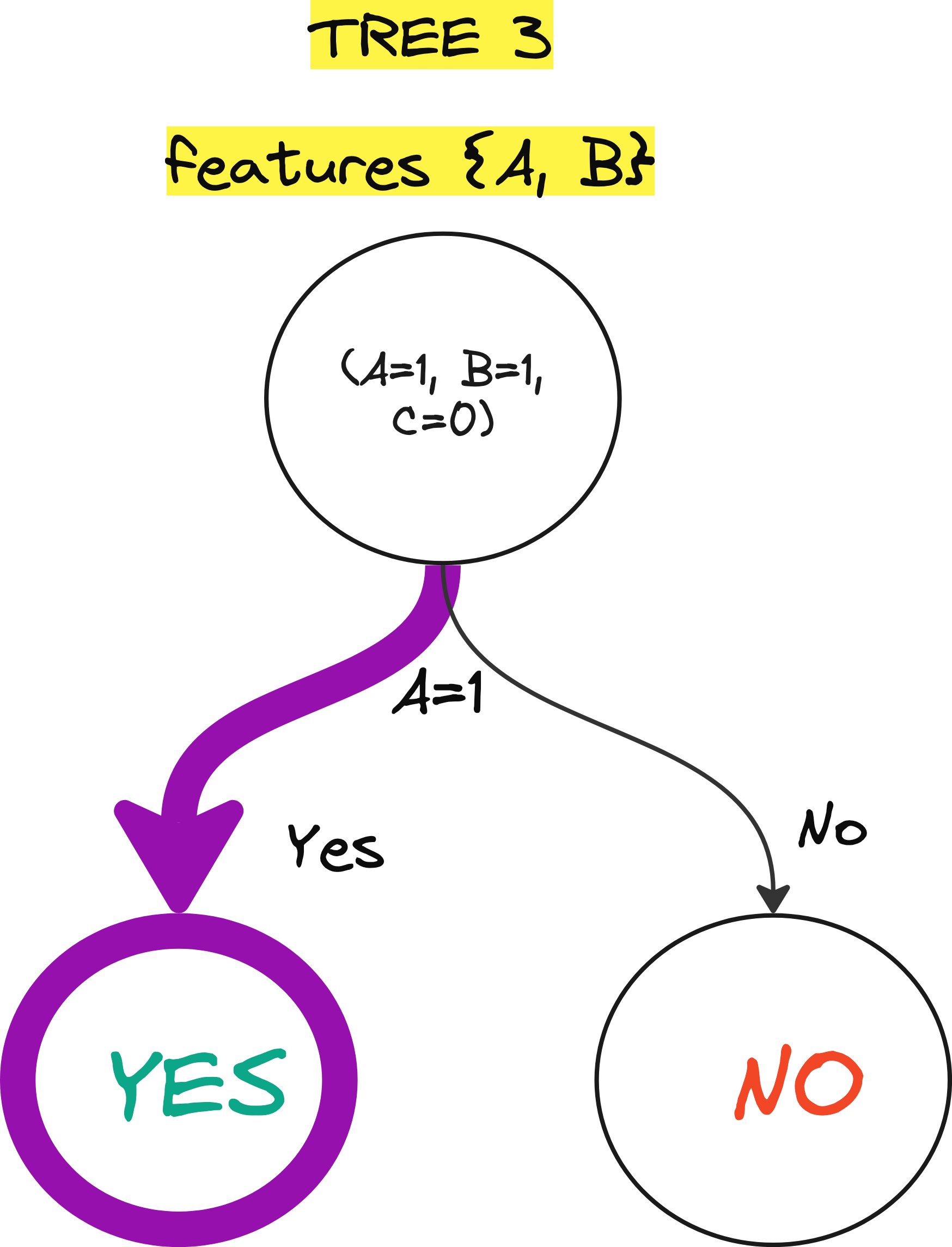
3. Tree 3 features {A, B}

Here are the 3 trees that are making YES or NO predictions.

Here are the trained trees.

Step 3: Prediction for a new instance

Suppose we want to classify a new instance: (A=1, B=1, C=0).

• Tree 1 (based on A, C) predicts YES because A=1.

• Tree 2 (based on B, C) predicts NO because B=1 & C=0.

• Tree 3 (based on A, B) predicts YES because A=1.

Step 4: Aggregation Using Majority Voting

We take a majority vote of the three trees:

• YES (Tree 1, Tree 3)

• NO (Tree 2)

Since Yes appears twice, the final prediction for the instance (A=1, B=1, C=0) is YES.

So what is the final verdict made by this random forest consisting of just 3 trees? It will say “YES”. Because in a democracy of 3 trees, two of them said yes and one said no.

A few points to note

In random forest:-

• For classification, it takes the majority vote from all trees.

• For regression, it takes the average of all tree outputs.

Why use random forest in the first place?

• Overcomes overfitting in decision trees.

• Handles missing values and noisy data well.

• Works with both categorical and numerical data.

• Reduces variance and bias using bagging (Bootstrap Aggregating).

Disadvantages of random forest

Random forest is definitely not the holy grail. This is the reason why other better models have evolved later. Specifically, random forest has the following issues.

❌ Computationally expensive, especially with large datasets.
❌ Not interpretable like a single decision tree.
❌ Requires tuning of hyper-parameters for optimal performance.
❌ Memory-intensive with many trees.

Lecture video

If you are interested to learn about random forest in detail, I have released an entire lecture on this topic on Vizuara’s YouTube channel. Please check this out. I am sure you are going to enjoy this lecture as much as I enjoyed making it.

Code implementation

Please NOTE: The below from scratch implementation is not in Python, it is in Julia. Why Julia? Because I made this article based on a lecture I recently taught as part of my course “Introduction to Machine Learning in Julia”. Personally I love Julia (programming language). Even if you are a hard-core Python fanatic, I still recommend you to dip your toes into Julia once. You won’t regret it. In the best case, you will discover the world of Scientific Machine Learning in Julia.

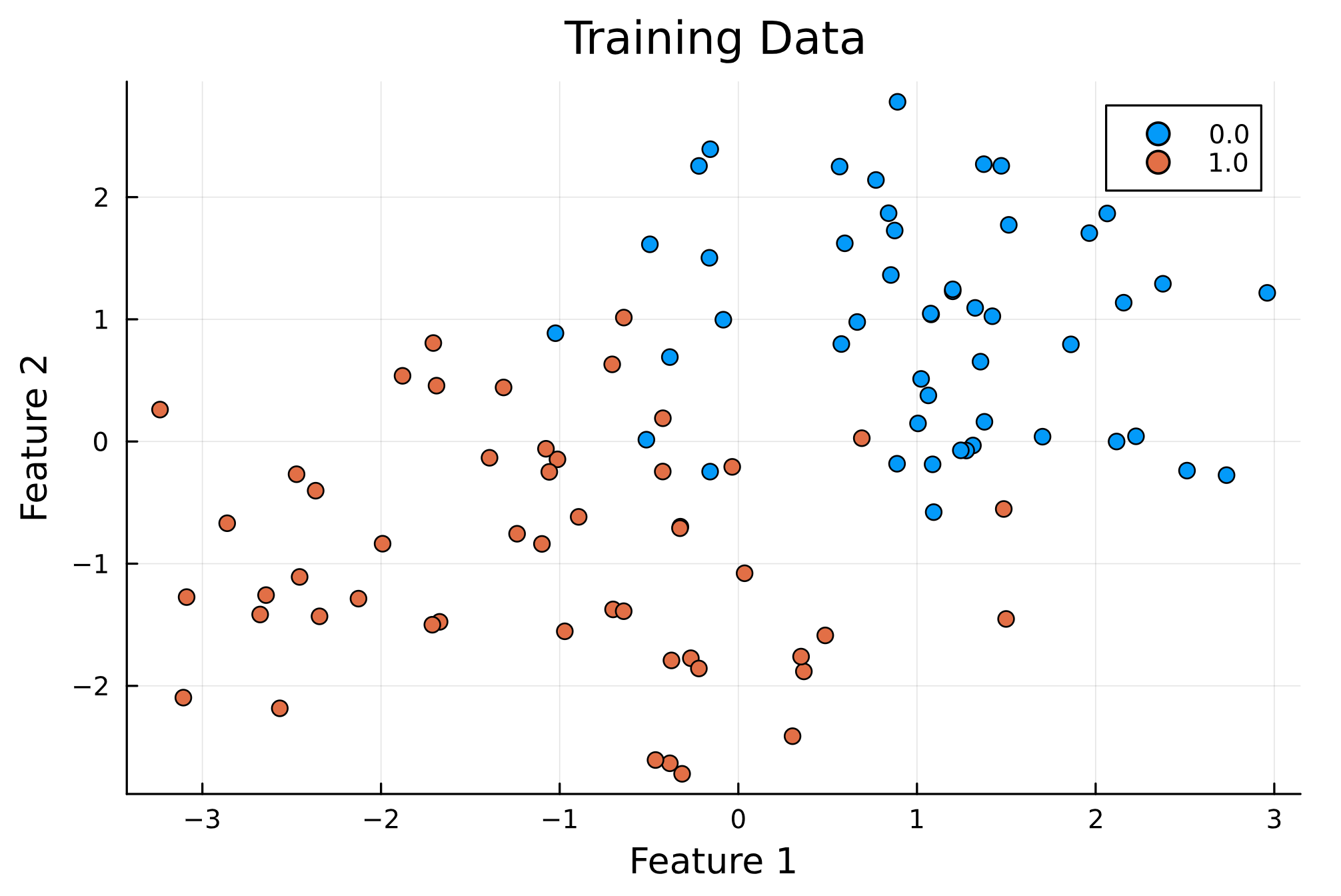
We will be implementing a random forest that can perform a binary classification on a dataset that has 2 features. The two images below show how the training data looks like and how the predictions would look like after implementing the code.

One more thing. Instead of throwing the code at you let us first brainstorm the steps needed to construct the code algorithmically.

1. First you need the dataset. You will have n data points. Each data points could have multiple features. They you will have a target variable corresponding to those n datapoints.

2. You have to split this dataset into two parts. Use 80% for training and 20% for testing.

3. You can assume that the labels are binary, meaning you are essentially performing a binary classification.

4. For ease of plotting the data on a 2D graph you can also assume that the dataset has only 2 features, that can be plotted on X and Y axis respectively.

5. The classification of the data (YES or NO) can be denoted using color.

6. Okay we are clear on the dataset. Now is the hard part. after splitting the dataset and getting the training dataset, what to do next.

7. We can define the number of trees in the forest and maximum depth of each tree and the minimum number of datapoints you need at a node before splitting the node into two branches.

8. We will need a variable to store the random forest.

9. We will need a variable to store all the trees in the forest.

10. For each tree, we need variables where we store the dataset at each node, the feature we are using to split that node and the threshold value of the feature we are using.

11. For every leaf node, we will need to know what prediction is being made. This can be done using “mode”. Whichever dataset dominates at the leaf node, you make classification into that category.

12. There is one more caveat. For random forest, every tree won’t get access to the entire dataset and the entire set of features. So, for each tree, we randomly sample a subset of data and subset of features.

13. How do we know which feature and what threshold to use at each node to split the subset of data using the subset of features available? Here we can use Information Gain (same as entropy reduction) or Gini impurity. In this code we will use Gini impurity.

14. So basically, at each node, have a look at the subset of data available, and enlist all possible features and all possible thresholds. Then iterate over the features and corresponding thresholds to figure out which feature and what threshold gives the maximum reduction in Gini impurity.

15. You recursively perform the node splitting operation until the depth of the tree reaches a pre determined value or the number of data points at a node becomes less than the minimum number of samples required at a node.

16. Once the tree building is finished, return the finished tree and store it in some variable where the forest is store.

17. Once every tree in the forest is finished, we are ready to make predications.

18. We can iterate over the test dataset. For every data point, let every tree make a prediction. How is the prediction made by an individual tree? There is a feature and threshold available at every node. So you traverse from parent node to the child node by following the feature value and feature threshold, until you reach a leaf node. Every leaf node has an already made prediction. So if a datapoint in the test data traverse along the branches of a tree to reach the leaf node, then we know the prediction.

19. Make these predictions for all trees.

20. Calculate the mode of all predictions. Use the “mode” of all predictions to say whether the collectively predicted (or voted) label for a given data point in the test data is YES or NO. This is where the democratic process happens.

21. Now you can read the code below.

Import required libraries

using Random
using StatsBase
using Plots
import StatsBase: mode

Gini impurity function

# Function to calculate Gini Impurity
gini_impurity(y) = 1 - sum((collect(values(countmap(y))) ./ length(y)) .^ 2)

Dataset splitting based on feature threshold

# Function to split dataset
function split_dataset(X, y, feature, threshold)
    left_idx = X[:, feature] .<= threshold
    right_idx = .!left_idx
    return X[left_idx, :], y[left_idx], X[right_idx, :], y[right_idx]
end

Finding the best split based on entropy reduction

# Function to find the best split
function best_split(X, y, feature_subset)
    best_feature, best_threshold, best_gini, best_split = nothing, nothing, Inf, nothing
    for feature in feature_subset
        thresholds = unique(X[:, feature])
        for threshold in thresholds
            X_left, y_left, X_right, y_right = split_dataset(X, y, feature, threshold)
            if length(y_left) == 0 || length(y_right) == 0
                continue
            end
            gini = (length(y_left) * gini_impurity(y_left) + length(y_right) * gini_impurity(y_right)) / length(y)
            if gini < best_gini
                best_gini = gini
                best_feature = feature
                best_threshold = threshold
                best_split = (X_left, y_left, X_right, y_right)
            end
        end
    end
    return best_feature, best_threshold, best_split
end

Individual node structure

# Decision Tree Node structure
mutable struct TreeNode
    feature::Union{Nothing, Int}
    threshold::Union{Nothing, Float64}
    left::Union{TreeNode, Nothing}
    right::Union{TreeNode, Nothing}
    prediction::Union{Nothing, Int}
end

Function to build the decision tree

# Function to build decision tree
function build_tree(X, y, depth, max_depth, min_samples)
    if length(y) <= min_samples || depth >= max_depth || gini_impurity(y) == 0
        return TreeNode(nothing, nothing, nothing, nothing, StatsBase.mode(y))
    end
    feature_subset = StatsBase.sample(1:size(X, 2), round(Int, sqrt(size(X, 2))), replace=false)
    feature, threshold, split = best_split(X, y, feature_subset)
    if isnothing(feature)
        return TreeNode(nothing, nothing, nothing, nothing, mode(y))
    end
    X_left, y_left, X_right, y_right = split
    return TreeNode(feature, threshold, build_tree(X_left, y_left, depth + 1, max_depth, min_samples), build_tree(X_right, y_right, depth + 1, max_depth, min_samples), nothing)
end

Function to predict for a new data point using a tree

# Function to predict using a tree
function predict_tree(node, x)
    if isnothing(node.feature)
        return node.prediction
    end
    return x[node.feature] <= node.threshold ? predict_tree(node.left, x) : predict_tree(node.right, x)
end

Building the random forest classifier

# Random Forest Classifier
mutable struct RandomForest
    trees::Vector{TreeNode}
end

Calling the random forest function

function RandomForest(n_trees, max_depth, min_samples)
    return RandomForest(Vector{TreeNode}(undef, n_trees))
end

Build tree using subset of data

# Function to fit Random Forest
function fit!(forest::RandomForest, X, y)
    n_samples, n_features = size(X)
    for i in 1:length(forest.trees)
        sample_idx = StatsBase.sample(1:n_samples, n_samples, replace=true)
        X_sample, y_sample = X[sample_idx, :], y[sample_idx]
        forest.trees[i] = build_tree(X_sample, y_sample, 0, 5, 2)
    end
end

Function to fit random forest

# Function to predict using Random Forest
function predict(forest::RandomForest, X)
    predictions = [predict_tree(tree, x) for tree in forest.trees, x in eachrow(X)]
    return [mode(predictions[:, i]) for i in 1:size(X, 1)]
end

Create training data

# Example usage
X_train = vcat(
    hcat(randn(50) .+ 1, randn(50) .+ 1),  # Cluster 1
    hcat(randn(50) .- 1, randn(50) .- 1)   # Cluster 2
)  # 100 samples, 5 features
y_train = vcat(zeros(50), ones(50))  # Binary labels
X_test = vcat(
    hcat(randn(10) .+ 2, randn(10) .+ 2),
    hcat(randn(10) .- 2, randn(10) .- 2)
)  # 10 test samples

rf = RandomForest(10, 5, 2)  # 10 trees, max depth 5, min samples 2
fit!(rf, X_train, y_train)

Function to print all the trees in the random forest

# Print number of trees in the forest
println("Number of trees in the forest: ", length(rf.trees))

# Function to print tree structure
function print_tree(node, indent="")
    if isnothing(node.feature)
        println(indent, "Predict: ", node.prediction)
    else
        println(indent, "Feature ", node.feature, " <= ", node.threshold)
        print_tree(node.left, indent * "  ")
        print_tree(node.right, indent * "  ")
    end
end

Print all the trees in the random forest

# Print all trees in the forest
for (i, tree) in enumerate(rf.trees)
    println("Tree ", i, ":")
    print_tree(tree)
    println()
end
predictions = predict(rf, X_test)

Scatter plot visualization of training data and predictions

# Visualizing Training Data
scatter(X_train[:, 1], X_train[:, 2], group=y_train, legend=:topright, title="Training Data", xlabel="Feature 1", ylabel="Feature 2")
display(scatter(X_train[:, 1], X_train[:, 2], group=y_train, legend=:topright, title="Training Data", xlabel="Feature 1", ylabel="Feature 2"))

# Visualizing Predictions
scatter(X_test[:, 1], X_test[:, 2], group=predictions, legend=:topright, title="Test Predictions", xlabel="Feature 1", ylabel="Feature 2")
display(scatter(X_test[:, 1], X_test[:, 2], group=predictions, legend=:topright, title="Test Predictions", xlabel="Feature 1", ylabel="Feature 2"))

# Evaluate accuracy on training set
y_train_pred = predict(rf, X_train)
correct = sum(y_train .== y_train_pred)
total = length(y_train)
println("Training Accuracy: ", correct / total * 100, "%")