If you have 96 attention heads, will you run 96 loops?

Deeply understanding multi-head attention with weight splits

and

Oct 30, 2025

When people first hear about attention mechanisms in transformers, they often imagine something very abstract. In reality, it is a beautifully logical and structured mathematical process that, once understood, gives you a clear picture of how large language models like GPT-3 or Vision Transformers process information. In today’s discussion, we are going to understand multi-head attention from its fundamental implementation and see how it can be made scalable using a concept known as weight splitting.

Revisiting the Basics of Multi-Head Attention

Let us begin with the basics. Imagine that you have a set of input tokens, each represented as a vector. These could be words in a sentence or image patches in a Vision Transformer. Each input token, say of dimension three, is transformed into three separate spaces using three distinct matrices known as WQ, WK, and WV, corresponding to queries, keys, and values.

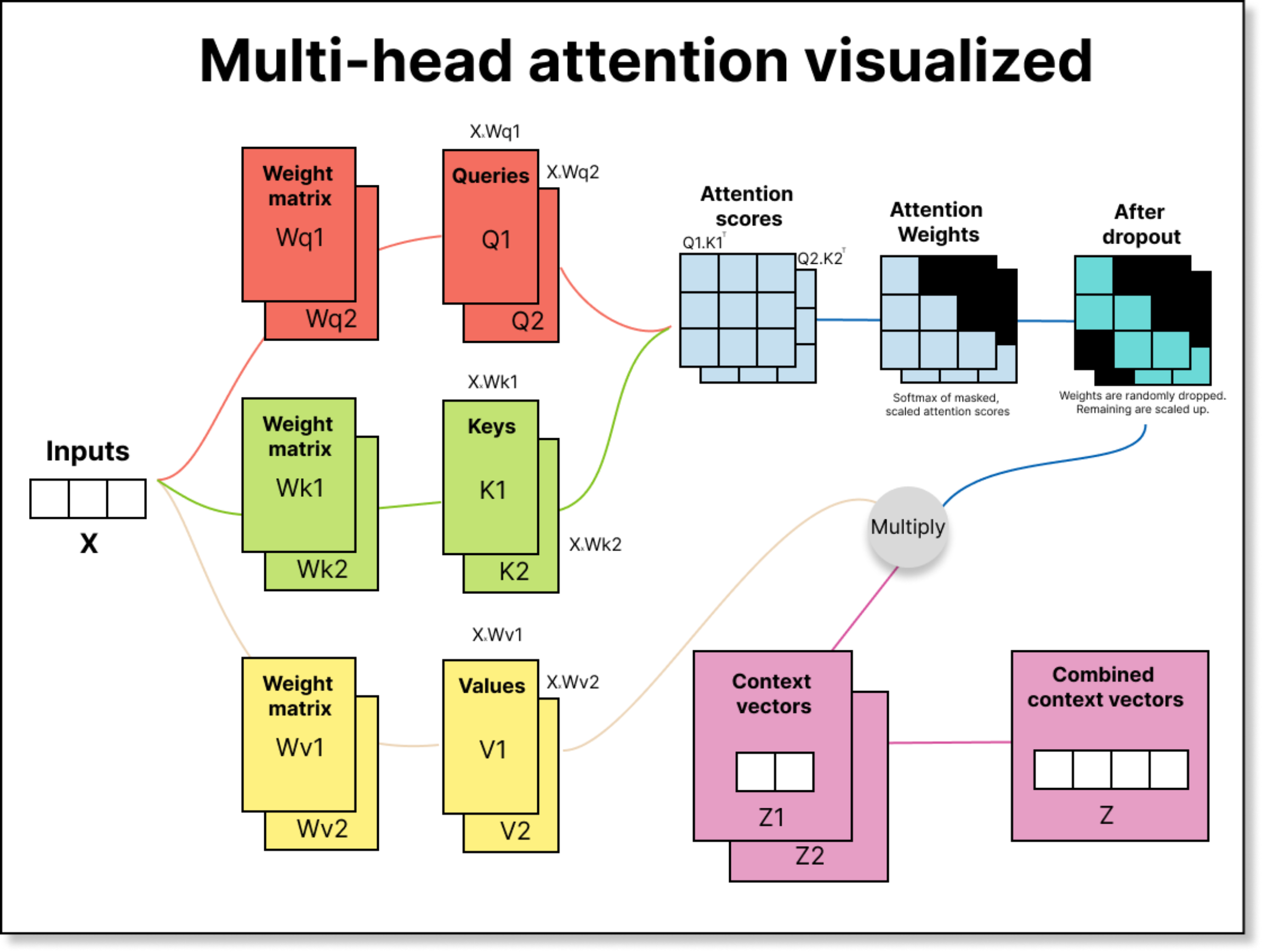
In a simple single-head attention mechanism, you would multiply your input matrix X (say of size 6 × 3, representing 6 tokens of 3 dimensions each) with these weight matrices of size 3 × 2 to obtain 6 × 2 query, key, and value matrices. You then compute attention scores by taking the dot product between the query and the transposed key, scale the result by 1 over the square root of the key dimension, apply masking and softmax to obtain attention weights, and finally multiply those weights with the value matrix to get context vectors.

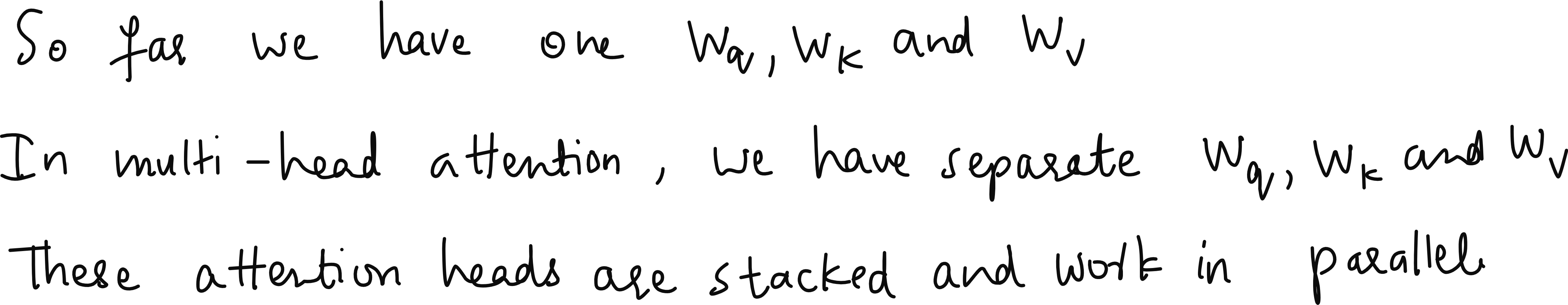
Now, multi-head attention extends this idea by having multiple such query-key-value projections. If you have two heads, you have two sets of WQ, WK, and WV. Each head works in its own subspace, and the outputs from all heads are concatenated to produce the final context representation.

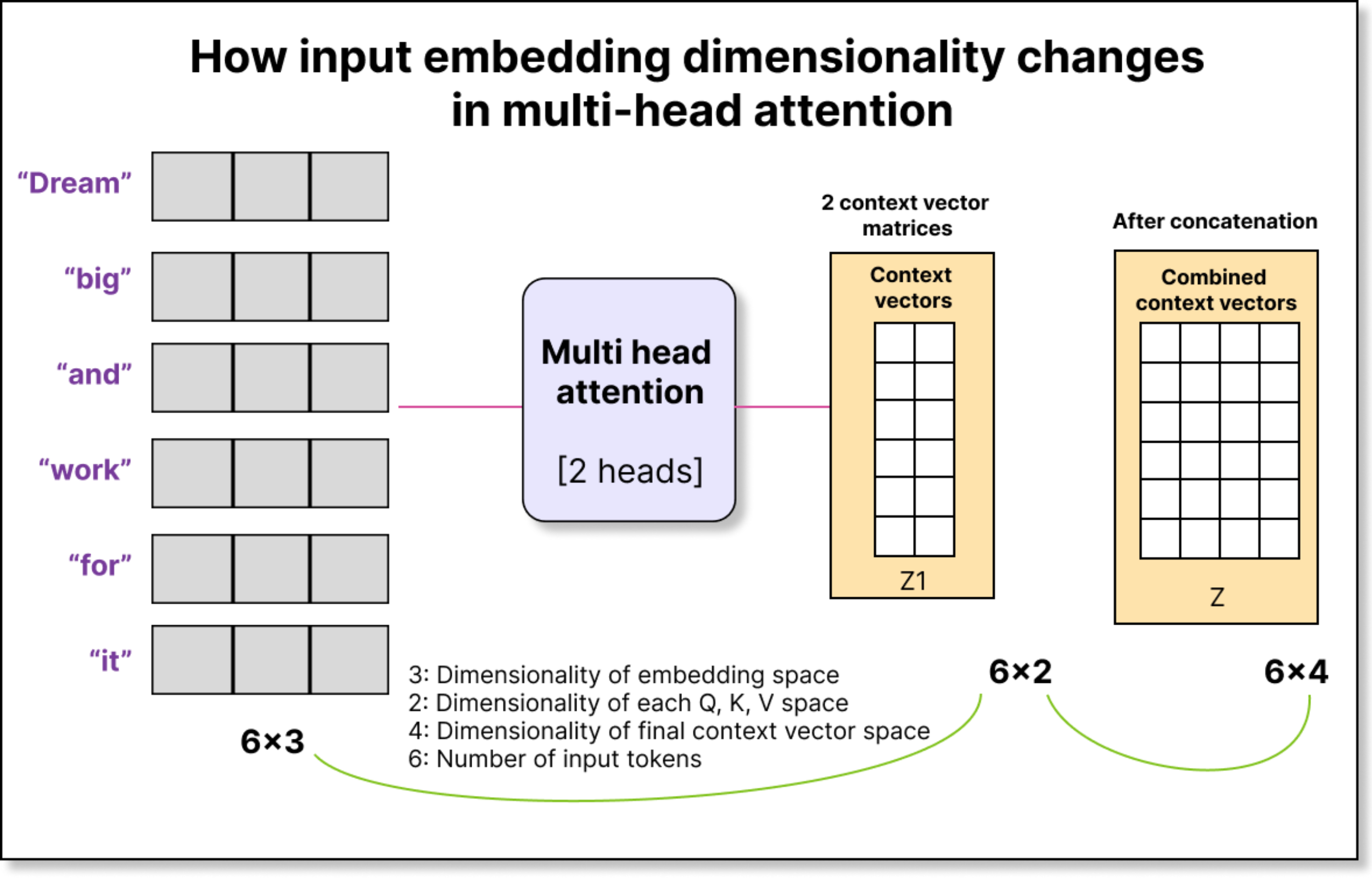
For example, if each head produces an output of dimension two and you have two heads, the concatenated output per token will have dimension four. Thus, from an input of 6 × 3, you can end up with an output of 6 × 4, where each token’s contextual representation now integrates information captured by multiple independent attention heads.

The Problem With the Naive Implementation

While this naive implementation works perfectly for a small model, it becomes inefficient for large models. For instance, GPT-2 small uses 12 attention heads, and GPT-3 uses 96. If you compute Q = X × WQ separately for each head, you are performing 96 separate matrix multiplications just for queries, and another 96 each for keys and values.

Matrix multiplication is fast, but looping over 96 separate heads creates serious inefficiencies. Python and PyTorch can handle vectorized operations efficiently, but looping through heads introduces unnecessary overhead and memory fragmentation.

Hence, a need arises to perform all these computations together in one go, in a single large matrix multiplication operation. This is where the idea of weight splitting comes in.

The Idea Behind Weight Splitting

Instead of maintaining 96 different weight matrices for the queries (one for each head), what if we had just one big weight matrix WQ that internally contained all of them?

Let us assume we want the final output dimension to be 6, and we have 3 attention heads. That means each head is responsible for a subspace of 6 ÷ 3 = 2 dimensions. Instead of having three separate WQ matrices of size 3 × 2, we can have a single WQ matrix of size 3 × 6. When you multiply X (6 × 3) with WQ (3 × 6), you get a 6 × 6 query matrix. You can then split this 6-dimensional space into three chunks, each corresponding to one head, using tensor reshaping operations.

This way, you perform only one matrix multiplication (X × WQ) instead of three (X × WQ1, X × WQ2, X × WQ3). You can do the same for keys and values. Once Q, K, and V are computed, you split them into smaller pieces, one for each head, and process them in parallel.

This method removes all for-loops from the implementation, replacing them with tensor reshaping and permutation operations, making the model highly scalable and GPU-efficient.

Visualizing the Dimensionality Step-by-Step

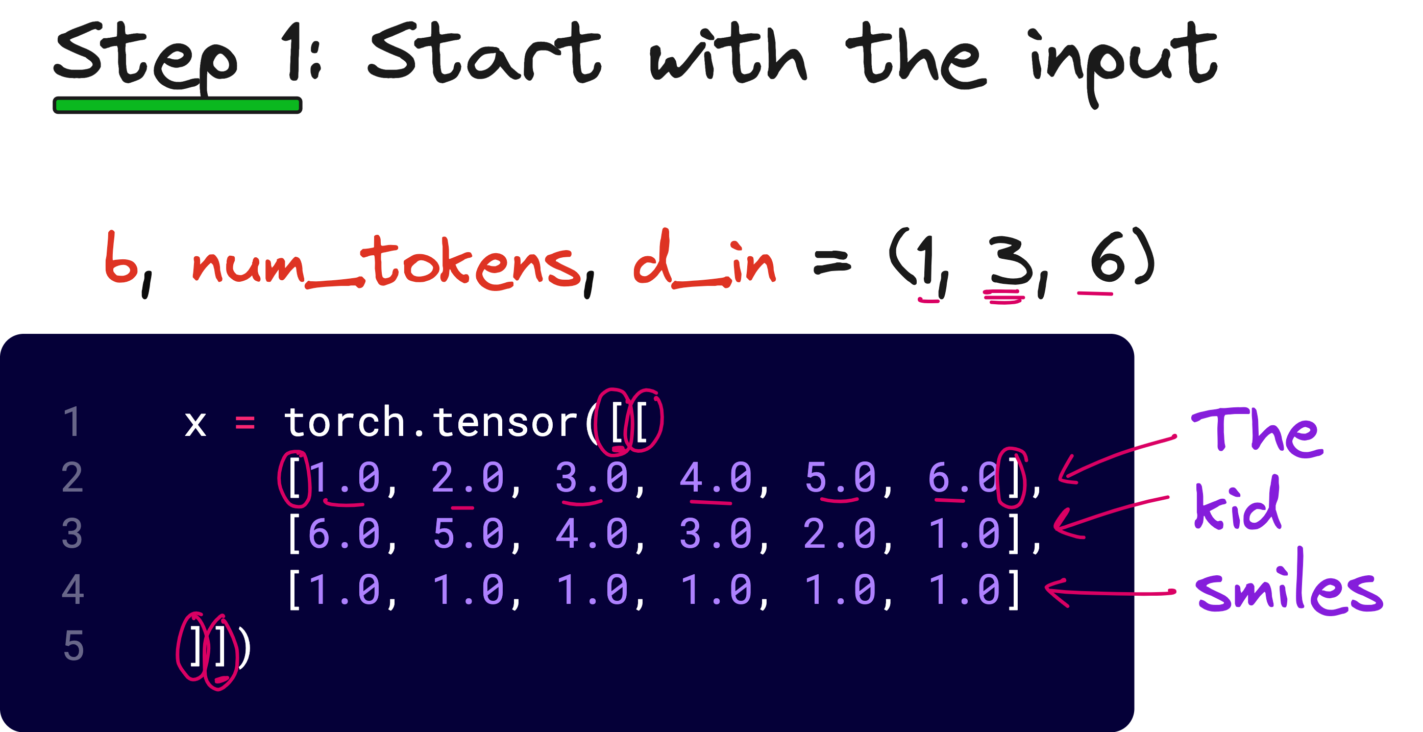
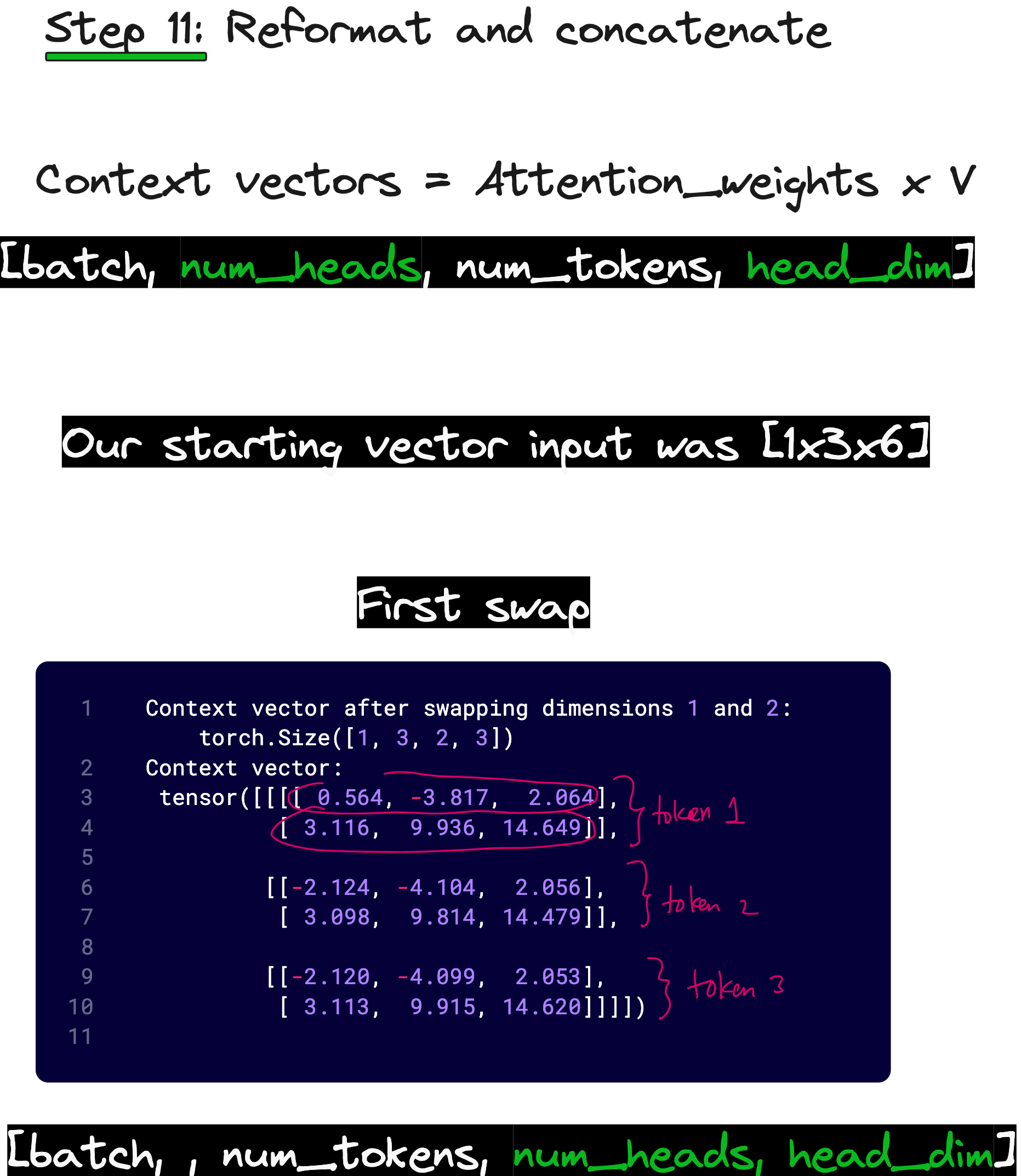
To understand this clearly, let us take an example where we have 3 input tokens, each of dimension 6, and we want 2 attention heads. Our input tensor X has shape (1, 3, 6), where 1 is the batch size, 3 is the number of tokens, and 6 is the embedding dimension.

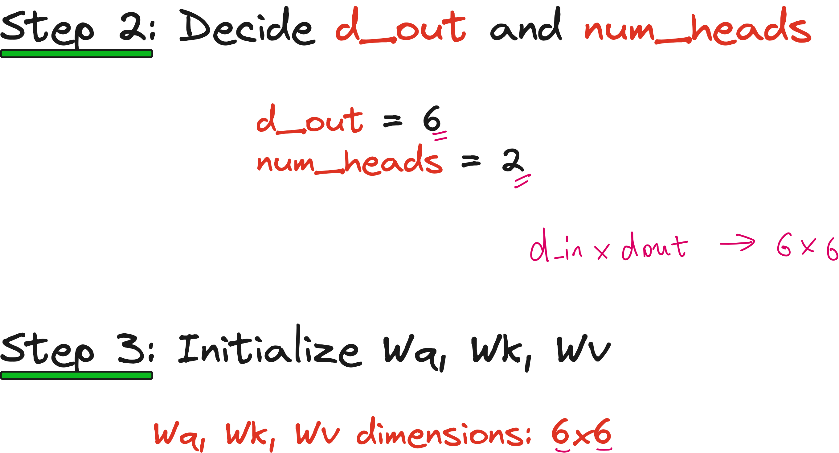
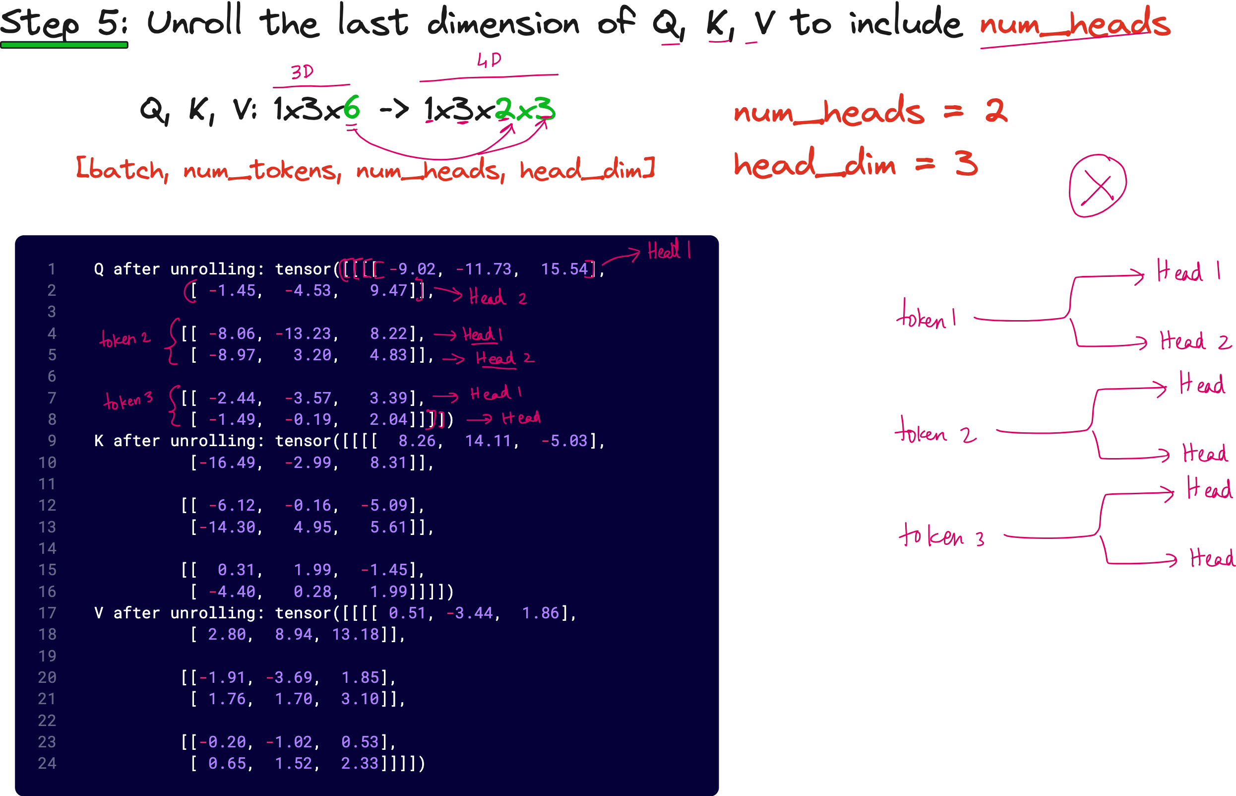
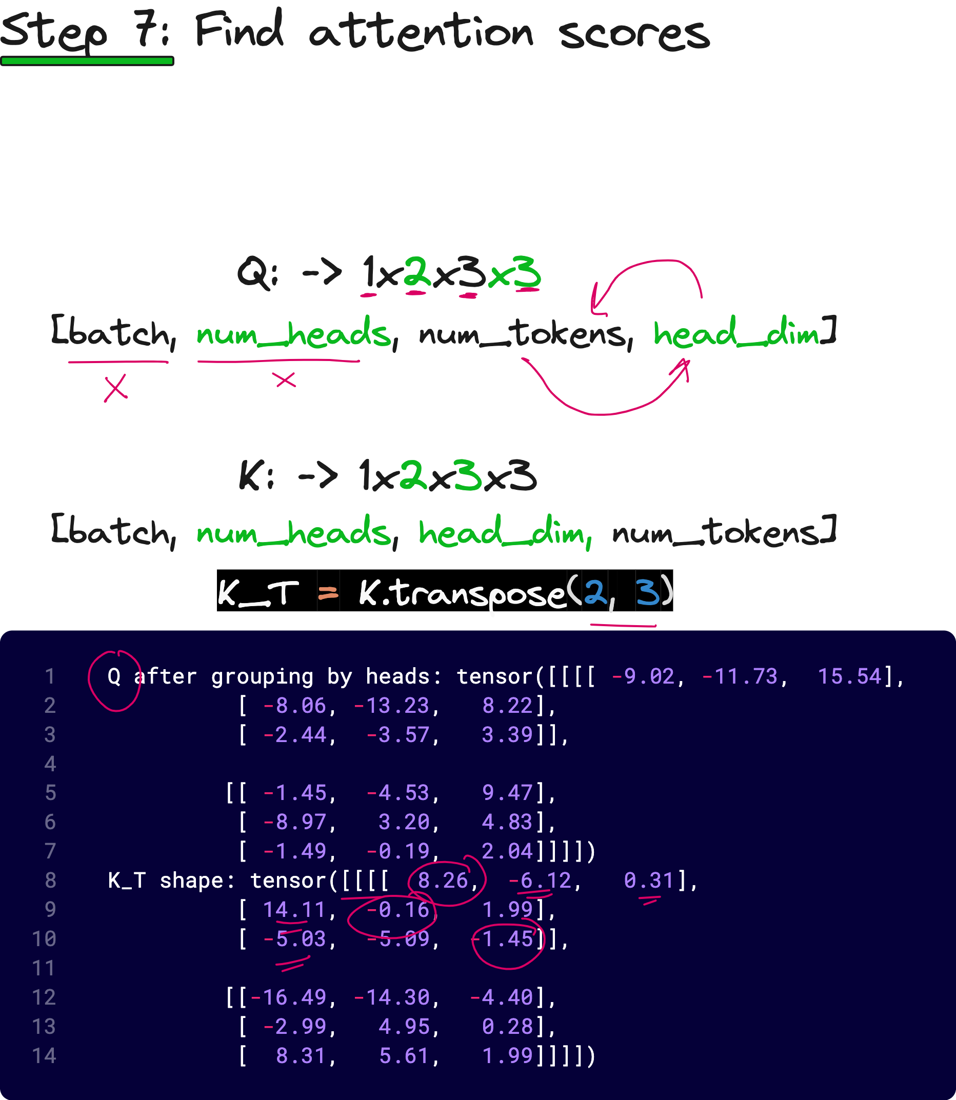
We multiply X with WQ of size (6 × 6) to obtain Q of shape (1, 3, 6). We then reshape this into (1, 3, 2, 3) — that is, batch size 1, 3 tokens, 2 heads, and 3 dimensions per head. This operation is known as unrolling the last dimension.

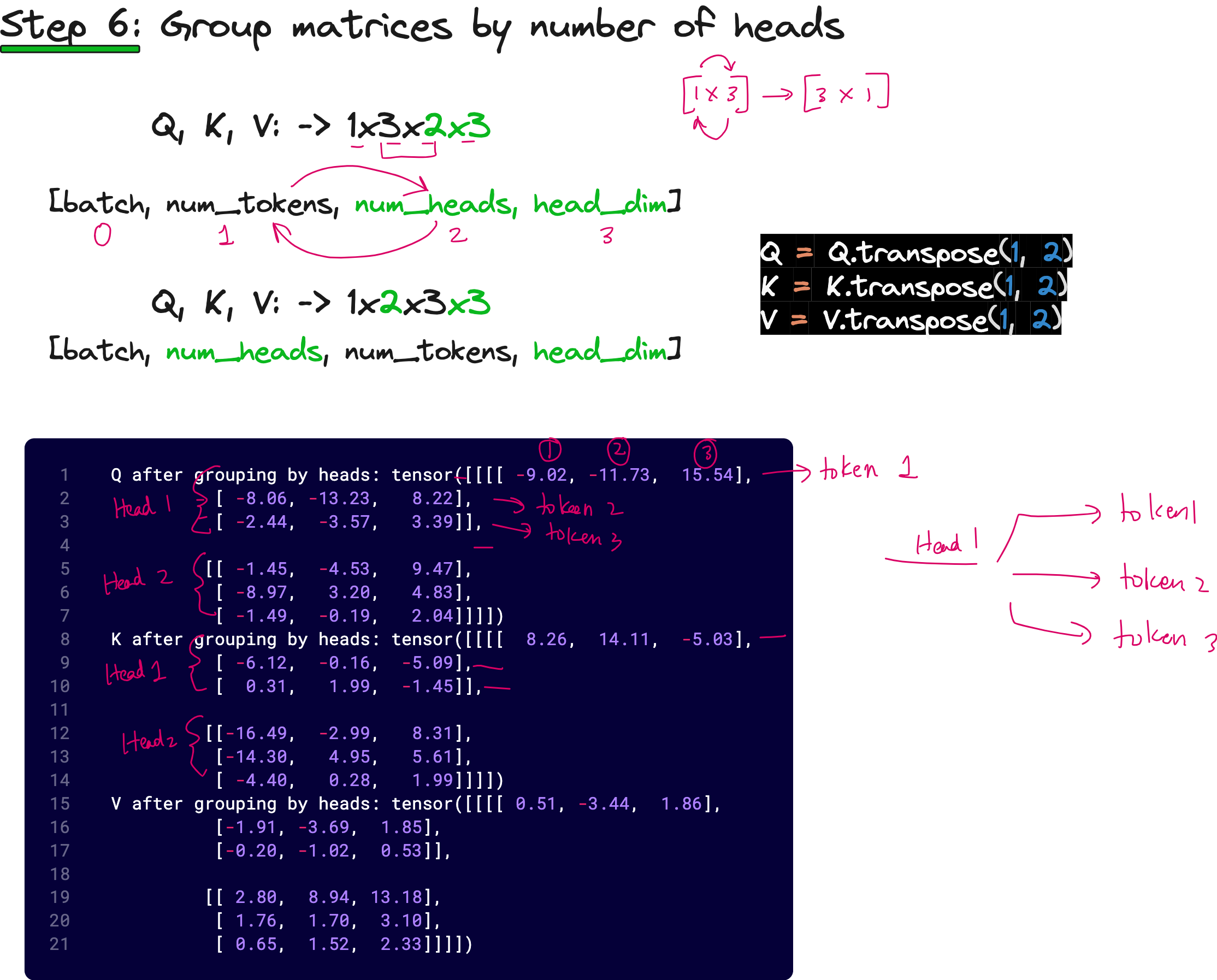
Now, we swap the second and third dimensions so that we have (1, 2, 3, 3) — one batch, two heads, three tokens, three dimensions per head. This rearrangement helps us group data based on heads rather than tokens, allowing easy computation of attention scores per head.

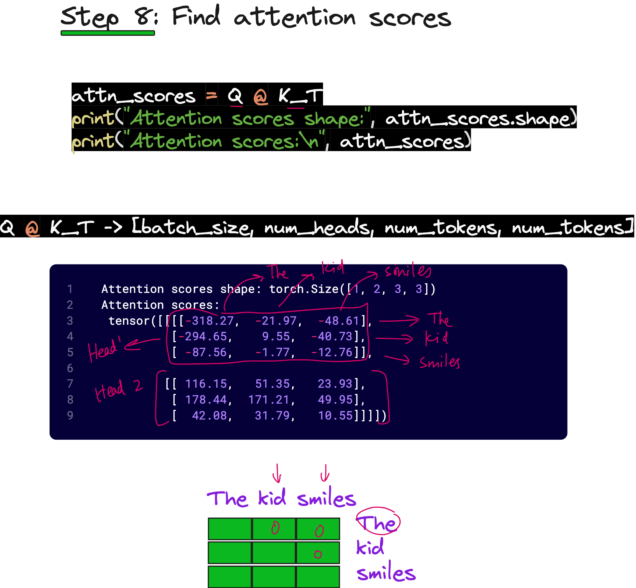
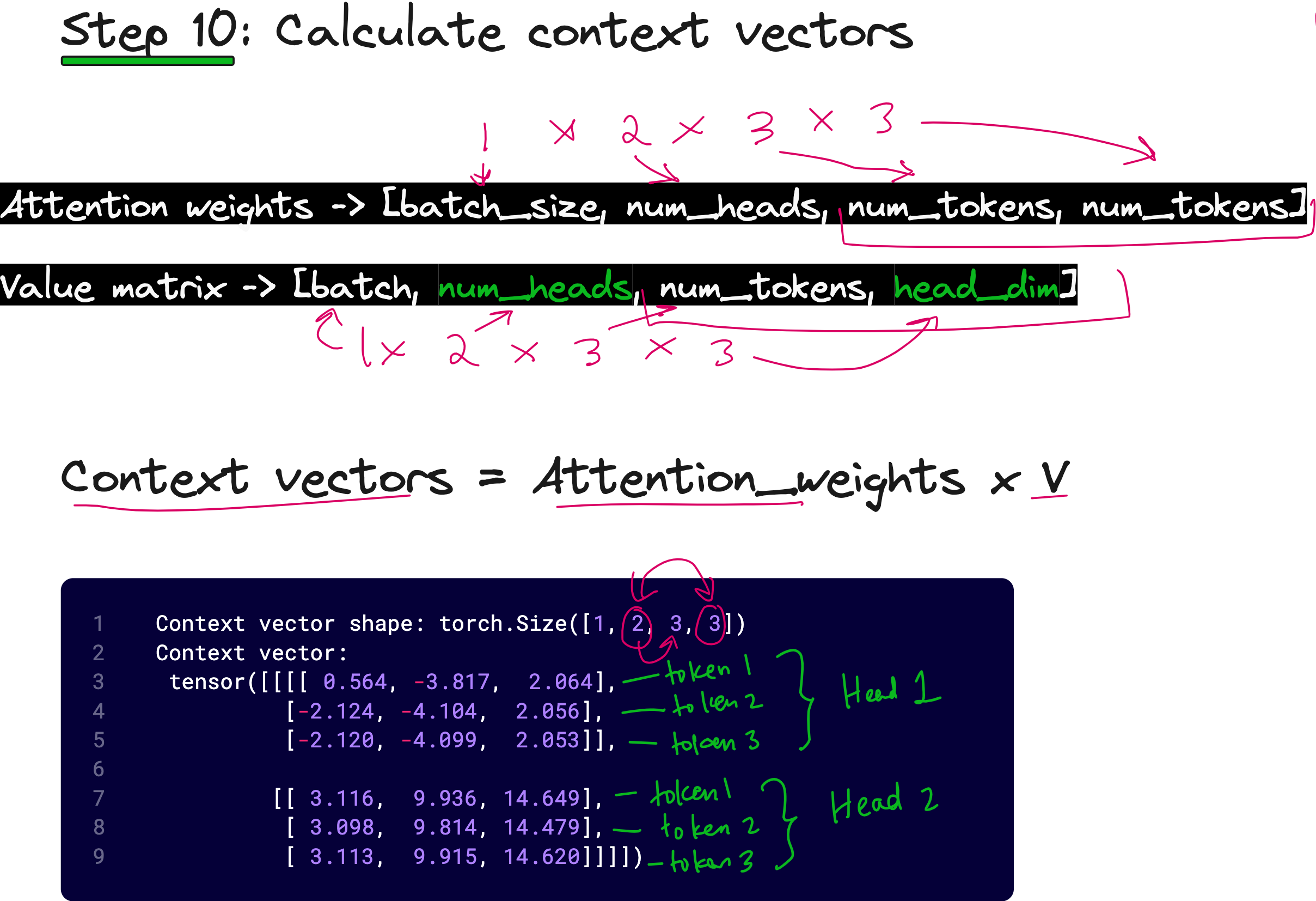
Next, for each head, we compute the attention scores by taking the dot product of Q and Kᵀ along the last two dimensions. The output will have shape (1, 2, 3, 3), representing attention scores for each head and each pair of tokens.

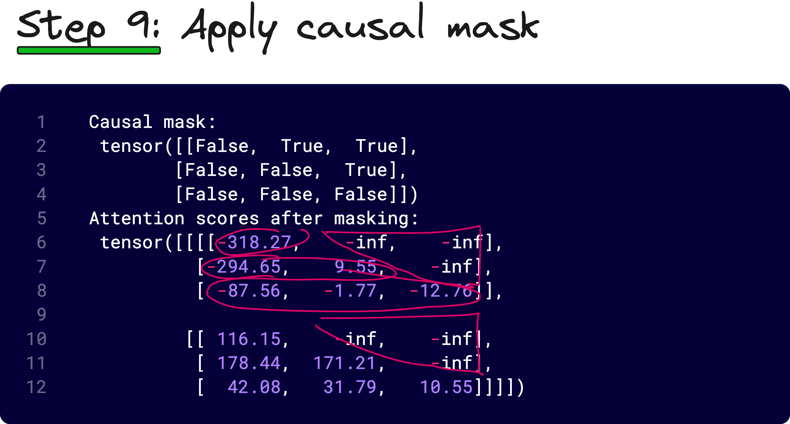
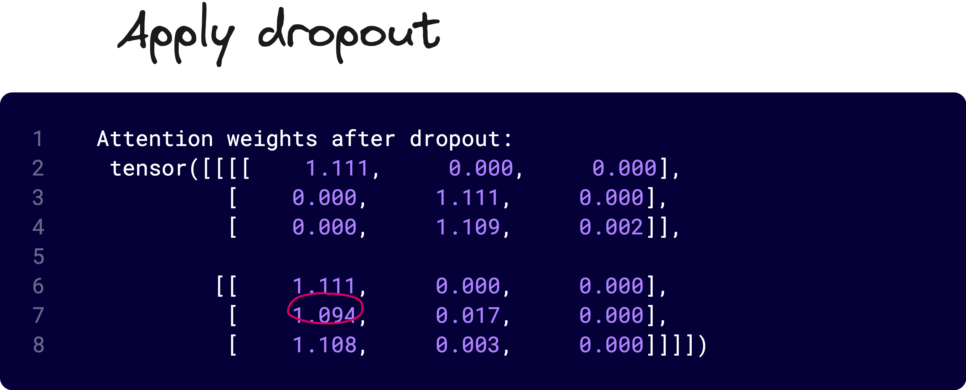
We then apply masking, scaling by 1/√dₖ, and softmax to convert these scores into attention weights. Optionally, dropout is applied to regularize the attention distribution.

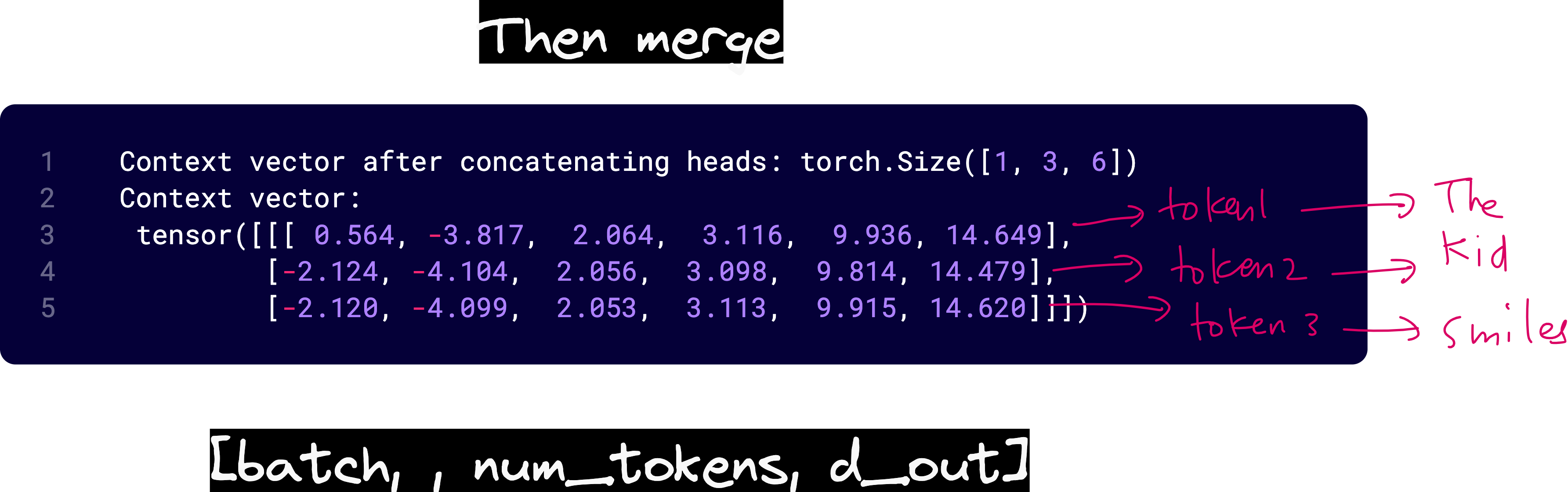
Finally, we multiply the attention weights with V to obtain context vectors of shape (1, 2, 3, 3). To merge all heads back together, we transpose dimensions again and reshape from (1, 2, 3, 3) to (1, 3, 6). Now we have the final context vectors corresponding to each token, with all head information fused.

Why Weight Splitting Matters

The entire process we just saw involves no for-loops. Every operation is a tensor operation, efficiently handled by GPUs. Even if you increase the number of attention heads to 96, the computational cost remains the same in terms of matrix multiplication calls.

This is the real strength of weight splitting. It allows transformers to scale to hundreds of attention heads while maintaining efficiency. Without it, multi-head attention would be prohibitively slow and memory-hungry, especially for large models like GPT-4 or Vision Transformers with high-resolution inputs.

Moreover, weight splitting makes the architecture elegant and uniform. Each operation can be expressed as a single large matrix multiplication followed by tensor reshaping, making both the implementation and debugging process much cleaner.

The Broader Picture

When you understand this flow — from naive multi-head attention with individual WQ, WK, and WV matrices to the efficient implementation with weight splitting — you begin to see how the transformer architecture achieves both scalability and parallelism.

Transformers are designed to take advantage of GPUs by using tensor operations rather than loops. This is not just an optimization trick, it is a fundamental design philosophy that makes these models viable for massive-scale training.

Whether you are building a text-based transformer or a vision transformer, the mathematics remains the same. The only difference lies in how you interpret the input tokens — words in the former, and image patches in the latter.

Conclusion

Multi-head attention is not merely a concept in deep learning theory. It is a remarkable engineering solution that allows models to attend to multiple subspaces of information simultaneously. And through weight splitting, we make this process computationally elegant and efficient.

If you are building your own transformer or even trying to understand how frameworks like PyTorch or TensorFlow implement them, this step-by-step understanding of shapes, tensor rearrangements, and dimensionality transitions will make the entire idea feel intuitive and logical.

Once you understand these details, you no longer see attention as a mystery. You see it as a clear, structured computation that can be extended, optimized, and even adapted to different modalities like images, text, or graphs with remarkable ease.