
How I Shipped an End-to-End ML Anomaly Detection System on the NYC Taxi Dataset (With CI/CD)
In this article , My aim is to explain how you can implement entire production ready project in Machine learning.


Table of content
Introduction
Repository Organization and Engineering Rationale
Data Ingestion and Reproducibility
LSTM Autoencoder for Time-Series Reconstruction
Training Pipeline and Artifact Generation
Batch and Streaming Inference with FastAPI
Model loading and scoring utilities
Batch endpoint (offline scoring)
Streaming endpoint (online scoring) and the “window availability” issue
MongoDB Logging
Visualization via Streamlit Dashboard
Monitoring: Prometheus-Compatible Metrics
Containerization and Local Orchestration
Continuous Integration and Continuous Delivery (CI/CD)
Execution Summary (Reproducible Runbook)
Limitations and Planned Extensions
1.Introduction
Most anomaly detection projects die in a notebook.
You train an autoencoder, plot reconstruction error, pick a threshold, and call it a day. But the moment you try to use the model like a real system, where data arrives one point at a time, where you need persistence, monitoring, and safe deployments, you realize the “ML part” was only 20% of the job.
So I built this project to answer a simple question:
What does a production-style anomaly detection pipeline look like end-to-end—training → packaging → streaming inference → dashboard → CI/CD?

This Article is based on the actual repo I implemented, using the NAB NYC Taxi time-series dataset (nyc_taxi.csv). I’ll explain the architecture, the reasoning behind key decisions, the “gotchas” (including the classic streaming bug), and how I wired it into a CI/CD pipeline that ships Docker images automatically.
What We are going to built throughout the article is :
A time-series anomaly detection system for NYC Taxi data that supports:
Offline training (LSTM Autoencoder)
Batch inference (score a whole sequence)
Streaming inference (score one datapoint at a time with a sliding buffer)
Persistent logging (MongoDB)
Dashboarding (Streamlit)
Metrics endpoint (Prometheus)
CI + CD pipelines (GitHub Actions + GHCR Docker image publishing)
And the best part: it’s runnable locally with Docker Compose.
2. Repository Organization and Engineering Rationale
A central design principle was to separate concerns (training, shared model definition, serving, infrastructure, evaluation, and visualization) into clear modules. This reduces coupling, simplifies testing, and enables CI/CD to operate on the serving component without requiring the entire training environment.
The repository structure is as follows:
nyc-anomaly-fixed/
├─ data/
│  ├─ download_nab.py                 # programmatic retrieval of NAB dataset (nyc_taxi.csv)
│  └─ nyc_taxi.csv                    # generated by download script (or provided)
│
├─ train/
│  ├─ config.yaml                     # training hyperparameters and thresholding policy
│  └─ train.py                        # training pipeline: preprocessing → training → artifacts
│
├─ common/
│  └─ model_arch.py                   # LSTM Autoencoder architecture shared by train & serve
│
├─ app/
│  ├─ config.py                       # environment-driven application settings
│  ├─ model.py                        # ModelWrapper: artifact loading and inference utilities
│  ├─ main.py                         # FastAPI service (batch + streaming endpoints)
│  └─ Dockerfile                      # container build for the inference service
│
├─ infra/
│  └─ docker-compose.yml              # local stack: API + MongoDB
│
├─ dashboard/
│  └─ streamlit_app.py                # visualization of time series + anomalies from MongoDB
│
├─ eval/
│  ├─ download_nab_labels.py          # optional retrieval of NAB anomaly windows/labels
│  └─ evaluate.py                     # evaluation utilities for sanity checking
│
├─ models/                            # generated artifacts consumed by the API
│  ├─ lstm_ae.pth
│  ├─ scaler.npz
│  ├─ threshold.txt
│  └─ model_meta.json
│
├─ tests/
│  └─ test_model_wrapper.py           # CI test scaffold (extensible)
│
├─ requirements.txt
├─ requirements-dashboard.txt
│
└─ .github/workflows/
   ├─ ci-cd.yml                       # CI: run tests on PR/push
   └─ cd.yml                          # CD: build & push Docker image to
This layout supports three important engineering requirements:
Reproducibility: training outputs are serialized into a stable artifact bundle.
Deployability: the service (
app/) depends only on artifacts and shared model code (common/).Auditability: predictions and scores are logged to a database rather than being ephemeral.
3. Data Ingestion and Reproducibility
The dataset is retrieved programmatically via data/download_nab.py, which ensures that a fresh clone of the repository can reproduce the input data without manual downloads. This is a modest but important practice: by treating dataset retrieval as part of the pipeline, the system becomes easier to validate in CI and easier for other users to reproduce reliably.
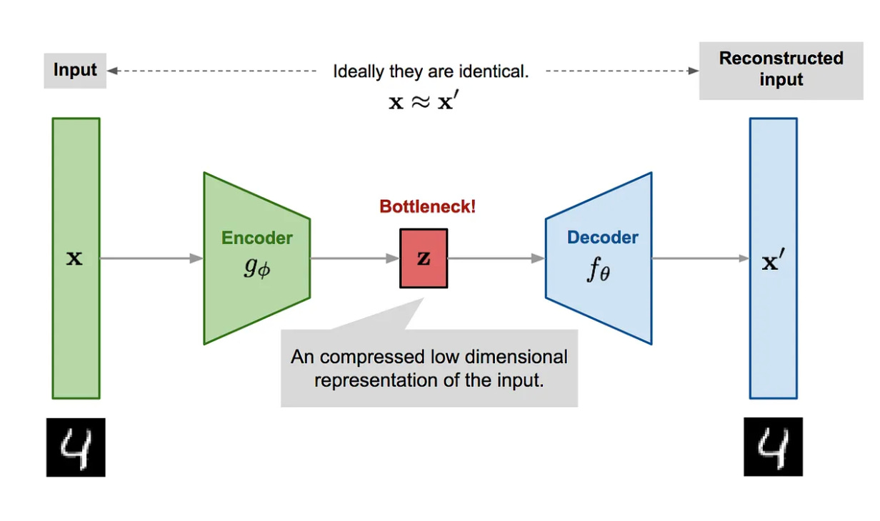
4. LSTM Autoencoder for Time-Series Reconstruction
4.1 Rationale
The core detector is an LSTM Autoencoder, implemented in common/model_arch.py. The underlying assumption is standard in reconstruction-based anomaly detection:
The model is trained primarily on typical (dominant) behaviour in the series.
At inference, windows inconsistent with learned structure yield higher reconstruction error.
Reconstruction error serves as an anomaly score.
This choice was guided by practical considerations: the model is sufficiently expressive for temporal structure, relatively straightforward to implement, and computationally feasible for repeated retraining during development.
4.2 Windowing
The training and inference pipelines operate on sliding windows, where each input to the autoencoder is a contiguous subsequence of length window_size (configured in train/config.yaml). Windowing is not merely a modelling detail; it is the key interface between raw streaming events and the model.
5. Training Pipeline and Artifact Generation
Training is executed from train/train.py, configured by train/config.yaml. The pipeline performs the following steps:
Load and select signal: read
nyc_taxi.csvand extract thevaluecolumn.Normalize: fit a scaler (saved as
scaler.npz) so inference uses identical preprocessing.Construct windows: generate overlapping windows to form training samples.
Train LSTM Autoencoder: optimize reconstruction loss over windows.
Compute reconstruction errors: evaluate window-level errors on representative data.
Derive a threshold: select an anomaly threshold using a percentile policy.
Save artifacts: serialize the model, scaler, threshold, and metadata.A simplified representation of the thresholding policy is:
# conceptual illustration of the training thresholding step
errors = reconstruction_errors_over_windows
threshold = np.percentile(errors, 85.0)   # configurable in train/config.yaml
5.1 Why artifact bundling matters
The training stage produces not only a model but a complete artifact bundle required for correct inference:
lstm_ae.pth— model weightsscaler.npz— normalization parametersthreshold.txt— anomaly thresholdmodel_meta.json— model metadata (notably window size and configuration)
This design avoids a common operational failure mode: deploying a model without its exact preprocessing and thresholding context.
6. Batch and Streaming Inference with FastAPI
a) Model loading and scoring utilities
Inference is encapsulated in app/model.py via a ModelWrapper, which loads the artifacts from models/ and exposes scoring functions. This is an intentional boundary: API code should not re-implement preprocessing or scoring logic.
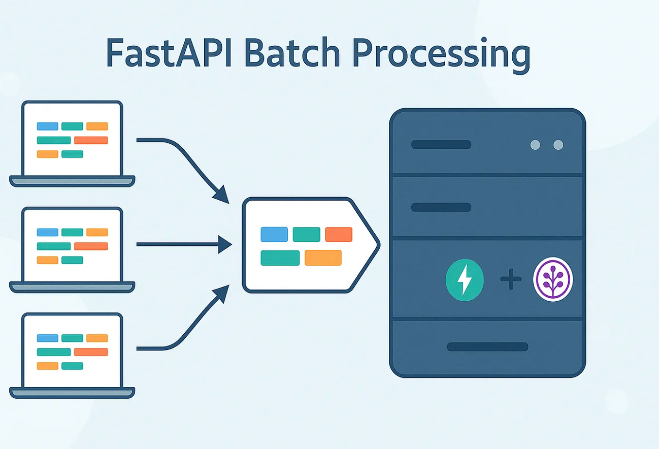
b) Batch endpoint (offline scoring)
The batch endpoint supports scoring of a provided sequence, enabling offline evaluation and experimentation. Batch scoring is particularly useful during development and for dataset-level assessments.
c) Streaming endpoint (online scoring) and the “window availability” issue
A central operational challenge in streaming anomaly detection is that a reconstruction model requires a full window to produce a meaningful score. If an API expects sequences but receives one point at a time, it may never accumulate enough observations to score—often leading to a misleading system that outputs “normal” indefinitely.
To address this, the service implements a streaming endpoint:
POST /predict_point
This endpoint maintains a per-stream buffer (indexed by stream_id) and returns a warm-up state until enough samples are available. Conceptually:
# conceptual illustration of streaming buffering
buffer[stream_id].append(value)

if len(buffer[stream_id]) < window_size:
    return {"label": "warmup"}

window = last_window(buffer[stream_id])
error = score(window)
label = "anomaly" if error > threshold else "normal"
This is an essential engineering feature: it aligns the inference contract with real telemetry settings, where observations arrive sequentially.
7. MongoDB Logging
The system logs each prediction to MongoDB (configured via app/config.py and orchestrated locally via infra/docker-compose.yml). Stored attributes include:
timestamp
stream identifier
observed value
reconstruction error
anomaly flag / label
inference mode (stream vs batch)
This logging enables:
retrospective debugging (why did we flag this point?)
dashboard visualization
downstream reporting and evaluation
auditability for operational use
8. Visualization via Streamlit Dashboard
The Streamlit application (dashboard/streamlit_app.py) queries MongoDB to display:
time-series trajectory
anomaly markers
reconstruction error over time
recent prediction records
The dashboard is intentionally lightweight; its function is to support rapid inspection and operational verification without requiring specialized observability infrastructure.
9. Monitoring: Prometheus-Compatible Metrics
The API exposes a metrics endpoint (/metrics) suitable for Prometheus scraping. At minimum, this supports:
counts of predictions by class (normal vs anomaly)
latency distributions for inference endpoints
This provides a practical bridge to production monitoring systems (Prometheus/Grafana) without overcomplicating the initial implementation.
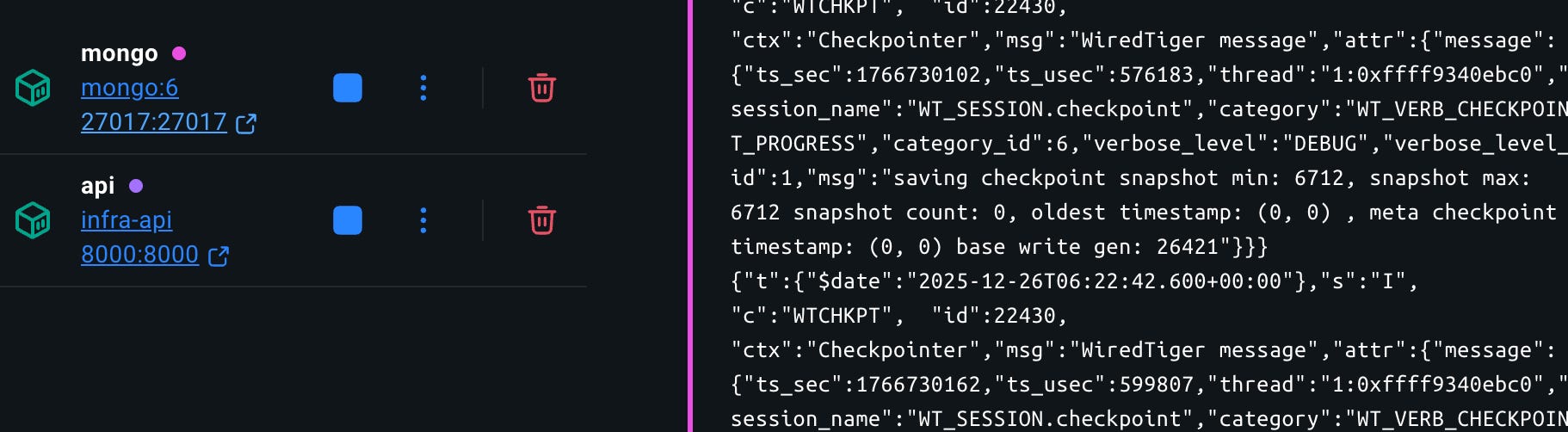
10. Containerization and Local Orchestration
The inference service is containerized via app/Dockerfile. Local orchestration is provided via infra/docker-compose.yml, which runs:
MongoDB
the FastAPI service
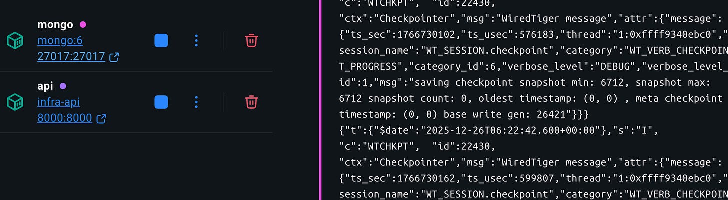
Above image shows , 2 services are live on docker , i.e Mongo for Database , API for the taking input request and output response
A notable design choice is that models/ is mounted into the service container. This permits:
retraining and artifact replacement without rebuilding the service image
clear separation between model development and service deployment
11. Continuous Integration and Continuous Delivery (CI/CD)
11.1 Continuous Integration
The CI workflow (.github/workflows/ci-cd.yml) executes on pushes and pull requests, running pytest. While the test suite is presently a scaffold, the workflow is correctly positioned to enforce:
artifact loading checks
scoring sanity checks
endpoint smoke tests
schema validation for request/response payloads
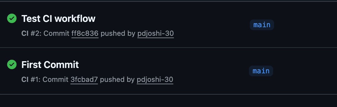
Demonstration of Continous Integration (C.I.) via GitHub Actions

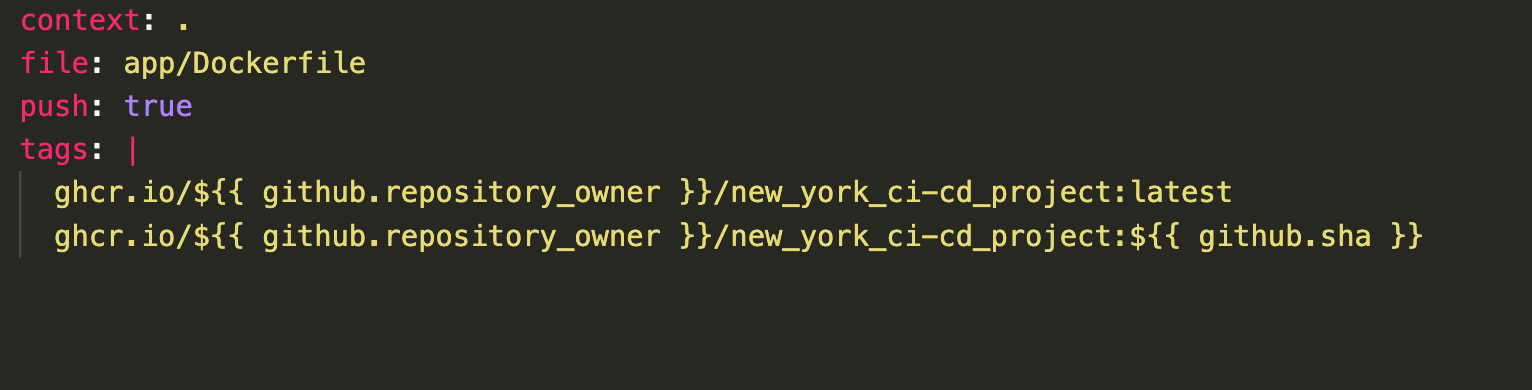
11.2 Continuous delivery : build and publish container images
The CD workflow (.github/workflows/cd.yml) builds and publishes the service container image to GitHub Container Registry (GHCR) on merges to main, tagging:
latestthe commit SHA
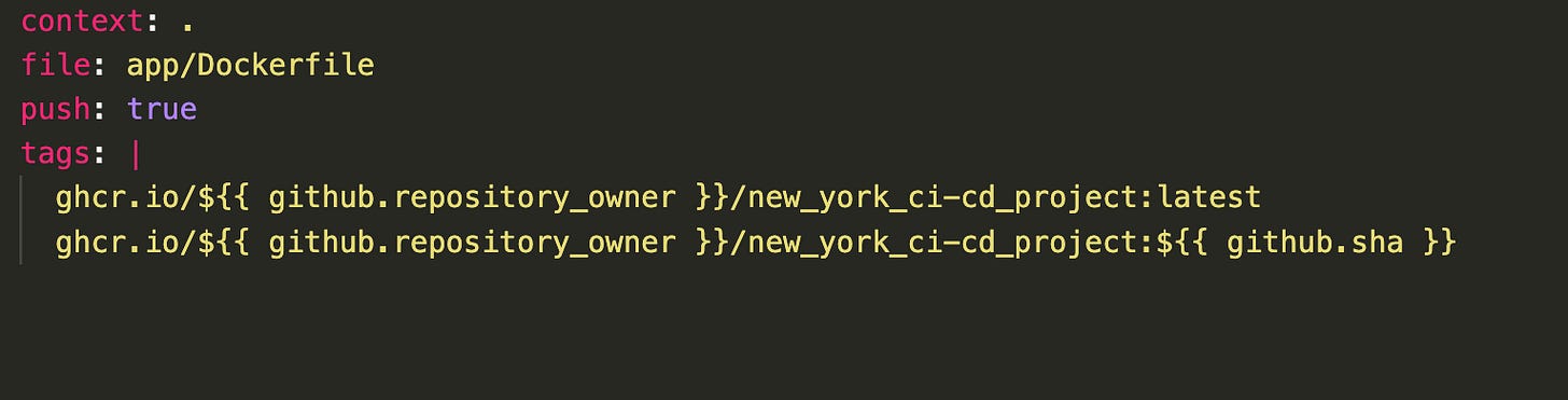
Actual Code Snippet from our Project. 
Demonstration of CI/CD both working correclty.
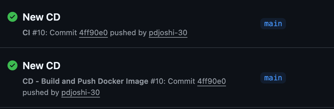
This ensures each release is reproducible, traceable, and readily deployable.
12. Execution Summary (Reproducible Runbook)
1) Download dataset
python data/download_nab.py --out data/nyc_taxi.csv
2) Train and generate artifacts
python train/train.py --config train/config.yaml
3) Run the local stack
docker-compose -f infra/docker-compose.yml up --build
4) Streaming inference
curl -X POST http://localhost:8000/predict_point \
  -H "Content-Type: application/json" \
  -d '{"stream_id":"default","value":23.1}'
5) Run the dashboard
streamlit run dashboard/streamlit_app.py
13. Limitations and Planned Extensions
While the system is end-to-end and deployable, several enhancements would be appropriate for production at scale:
Distributed streaming state: replace in-memory buffers with Redis to support multiple API replicas.
Model versioning: store artifact version/commit hash in prediction logs.
Robust evaluation: incorporate NAB label windows and compute precision/recall/F1 under standardized protocols.
Drift monitoring: track rolling distributions of reconstruction error and raw values.
Deployment automation: extend CD to deploy to a managed runtime (Cloud Run, ECS, Kubernetes).
Conclusion
This project demonstrates that effective anomaly detection requires both modelling and systems engineering. The LSTM Autoencoder provides a principled reconstruction-based detector, but the distinguishing contribution of the implementation is the operationalization: artifact bundling, streaming-safe inference, persistence, observability hooks, containerization, and automated CI/CD.
To know more about project and implementation detail please watch the video