
How I implemented PINNsformer Scratch??
In this article, we visit PINNsFormer, a Transformer-based physics-informed framework that blends attention mechanisms with wavelet activations to model complex spatiotemporal dynamics.


Table of Contents
Introduction
Architecture Overview
Pseudo Sequence Generator (PSG)
Spatio-Temporal Mixer
Encoder–Decoder Transformer
Wavelet Activation Function
Sequential Loss Function
Key Implementation Insights
Wavelet Activation Function
Inside the Transformer Core
Challenges Faced During Implementation
Comparison of Implemented Results with Reference Results
1D Reaction Equation
1D Wave Equation
Navier Stokes Equation
Why PINNsFormer Beats Classical PINNs
Broader Implications
Summary
1. Introduction
It started on a quiet evening when I was casually browsing through recent developments in Scientific Machine Learning. I wasn’t looking for anything specific, just exploring, the way you do when curiosity takes over. And then a title froze my scroll: PINNsFormer. A Transformer-based physics-informed architecture? With wavelet activations? Solving PDEs? I clicked instantly.
As I skimmed the paper, something about it pulled me in. For years, MLP-based PINNs had been my go-to, yet I’d seen them struggle slow convergence, unstable training, and a tendency to completely miss complex spatiotemporal patterns. But this paper offered a different vision: a fusion of attention mechanisms with the mathematical structure of physics. It felt like someone finally asked the same question I had been thinking for months: What if we brought the power of Transformers into the physics world?
That curiosity quickly turned into obsession. Instead of just reading the paper, I made a decision that both excited and terrified me I would implement the entire PINNsFormer architecture from scratch. No shortcuts, no blind copying. Just me, the paper, and the challenge.
The first few days were rough. The model diagram looked elegant on paper, but translating it into working code was a maze. The wavelet activation block didn’t behave the way I expected. The training loop kept exploding. And bridging the gap between the theoretical PDE constraints and attention-based representations felt like solving a puzzle with missing pieces.
But iteration by iteration—cross-checking equations, digging into their GitHub repo, fixing shape mismatches at 2 AM things slowly began to click.
Then came the breakthrough. The first time I plotted the predicted solution and it aligned almost perfectly with the ground truth, I realized: this architecture isn’t just hype—it works. I went on to test three of the PDE examples they showcased, and each time, the model captured dynamics that standard PINNs often fail to learn.
That journey from discovery to struggle to successful replication is what inspired this article.
In the sections ahead, I’ll break down PINNsFormer, share what worked (and what didn’t), and show you how this architecture pushes the boundaries of physics-informed learning.
2. Architecture Overview
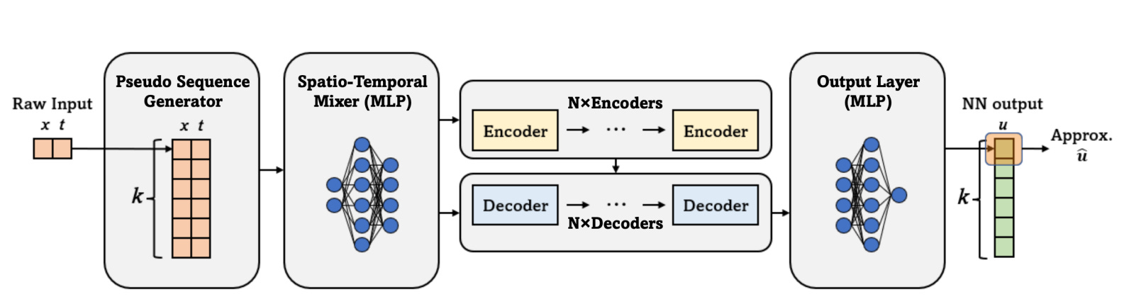
At its core, PINNsFormer rethinks the architecture of physics-based learning. Instead of treating each spatiotemporal point independently, it introduces the concept of pseudo-sequences, enabling temporal reasoning akin to time-stepping schemes in numerical solvers.
a) Pseudo Sequence Generator (PSG)
This module converts each pointwise input [x,t] into a pseudo-sequence such as [x,t],[x,t+Δt],…,[x, t+(k−1)Δt]. By transforming static inputs into sequences, the PSG allows the model to capture temporal dependencies and causal dynamics that standard PINNs overlook.
b) Spatio-Temporal Mixer
The mixer embeds low-dimensional spatial and temporal features into a high-dimensional latent space, enriching the data representation. This step helps the model encode complex relationships between space and time before passing them into the Transformer layers.
c) Encoder–Decoder Transformer
At the heart of the architecture lies the Transformer block.
The encoder captures global dependencies across pseudo-sequences, while the decoder focuses on selective local interactions.Through multi-head attention, this layer enables the network to learn both broad trends and fine-grained temporal behavior efficiently.
d) Wavelet Activation Function
Instead of conventional activations like ReLU or tanh, PINNsFormer uses a wavelet-inspired activation:
ω1sin(x)+ω2cos(x)This activation is smooth, differentiable, and Fourier-like providing stable gradients and better approximation of oscillatory physical dynamics.
e) Sequential Loss Function
Finally, PINNsFormer applies a physics-based loss function sequentially over pseudo-timesteps.
By enforcing residual, boundary, and initial condition losses at each step, the model maintains physical consistency across time and achieves smoother convergence.
This design allows PINNsFormer to treat PDE solutions as evolving temporal trajectories rather than static pointwise mappings.
3. Key Implementation Insights
a) Wavelet Activation Function
I decided to implement the entire PINNsformer architecture from scratch after going through the paper. I faced difficulties at the start but later, after iterating through the paper and their GitHub repository, I managed to get results and worked on three of the examples they tested. The idea of the wavelet function fascinated me, the authors didn’t use typical tanh or ReLU, but rather they developed their own custom activation function, Wavelet, which turned out to be very effective for this task.
class WaveAct(nn.Module):
    def __init__(self):
        super(WaveAct, self).__init__()
        self.w1 = nn.Parameter(torch.ones(1), requires_grad=True)
        self.w2 = nn.Parameter(torch.ones(1), requires_grad=True)

    def forward(self, x):
        return self.w1 * torch.sin(x)+ self.w2 * torch.cos(x)
The WaveAct class defines a custom activation function that combines sine and cosine transformations with learnable parameters. Inside the class, two trainable weights, w1 and w2, are initialized as ones and optimized during training. In the forward pass, the function computes y = w1 * sin(x) + w2 * cos(x), effectively creating a flexible wave-based activation. Since both sine and cosine are smooth and periodic, this combination produces a continuous and differentiable transformation that adapts as the network learns, allowing it to model nonlinear and oscillatory patterns more effectively than static activations like ReLU or Tanh.
Mathematically, this activation can be seen as a generalized sinusoidal function of the form Asin(x+ϕ), where the amplitude A and phase shift ϕ depend on the learned parameters w1 and w2. This means the activation dynamically adjusts its waveform during training, enabling the network to better capture periodic behaviors in data. While this flexibility can enhance representation power, it may also introduce instability if the learned weights cause excessive oscillation, making proper initialization or regularization important for stable learning.
b) Inside the Transformer Core
Initially, it took me some time to understand how to integrate a Transformer architecture for predicting the solutions of PDEs. Most of my prior experience with Transformers was in language and vision tasks, where self-attention and multi-head attention are applied differently. However, as I began implementing the model step by step, the underlying concept gradually became clearer. One key realization I gained through this process is that the best way to truly understand any algorithm is to implement it yourself the challenges you encounter along the way significantly deepen your intuition and comprehension of how the model actually works.
class PINNsformer(nn.Module):
    def __init__(self, d_out, d_model, d_hidden, N, heads):
        super(PINNsformer, self).__init__()

        self.linear_emb = nn.Linear(2, d_model)

        self.encoder = Encoder(d_model, N, heads)
        self.decoder = Decoder(d_model, N, heads)
        self.linear_out = nn.Sequential(*[
            nn.Linear(d_model, d_hidden),
            WaveAct(),
            nn.Linear(d_hidden, d_hidden),
            WaveAct(),
            nn.Linear(d_hidden, d_out)
        ])

    def forward(self, x, t):
        src = torch.cat((x,t), dim=-1)
        src = self.linear_emb(src)

        e_outputs = self.encoder(src)
        d_output = self.decoder(src, e_outputs)
        output = self.linear_out(d_output)
        return output
The PINNsformer class defines the complete architecture that combines Transformer-based sequence modeling with physics-informed learning. The model begins by embedding spatial and temporal inputs (x, t) using a linear layer that projects the 2D input into a higher-dimensional feature space (d_model). This embedding is then passed through an encoder–decoder Transformer, where the encoder captures global spatiotemporal dependencies across the pseudo-sequences, and the decoder selectively focuses on relevant temporal interactions. Together, these layers allow the network to learn long-range correlations and causal dynamics in the data, which are essential for accurately solving PDEs that evolve over time.
After the Transformer layers, the model employs a multi-layer output head (linear_out) that integrates the custom WaveAct activation function. This component transforms the encoded features into the final output while leveraging the smooth, oscillatory nature of WaveAct to model continuous and periodic physical patterns effectively. The repeated use of WaveAct between linear layers enhances the network’s ability to approximate complex solution surfaces governed by PDEs. Overall, the PINNsformer architecture elegantly merges physics constraints, attention mechanisms, and wavelet activations to form a data-efficient and physically consistent model for solving scientific problems.
4. Challenges Faced During Implementation
The first major challenge I faced during implementation was related to training compatibility and performance. The authors had used different CUDA versions for their experiments, whereas I was initially using a standard CUDA setup with a T4 GPU on Google Colab. To accelerate training and ensure smoother execution, I switched to an A100 GPU, which provided a default CUDA configuration optimized for deep learning workloads. This significantly improved the training efficiency and reduced computational bottlenecks.
Another critical aspect was hyperparameter tuning. My initial runs produced results that were far less accurate than those reported in the paper, with a considerable error gap. After experimenting with several parameters, such as the number of attention heads, learning rate, and the depth of hidden layers, I was eventually able to reproduce results that closely matched the paper’s benchmarks. This process reinforced the importance of hyperparameter tuning as a core skill for any machine learning engineer.
For the Navier–Stokes example, even with the A100 GPU, the training time remained substantial. This is understandable, as combining physics-based constraints with Transformer architectures introduces significant computational complexity. Such models, while powerful and expressive, inherently demand more resources and time to train effectively.
5. Comparison of Implemented Results with Reference Results
I experimented with the PINNsFormer architecture on three standard PDEs, the 1D Reaction Equation, the 1D Wave Equation, and the Navier–Stokes Equation. I selected these specific cases to directly compare my results with those reported in the original paper, allowing me to validate the correctness and consistency of my implementation.
Here are the results:
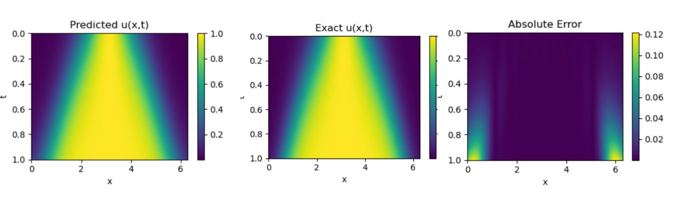
1D Reaction Equation
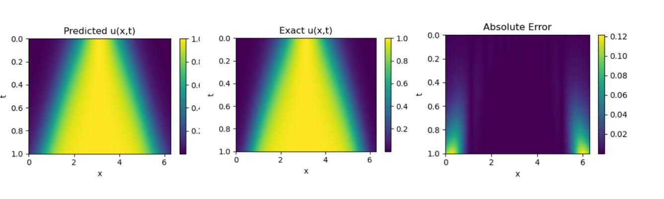
PINNsformer result on 1D Reaction Equation

We can observe an excellent alignment between the predicted and exact solutions, demonstrating the effectiveness and accuracy of the PINNsFormer architecture. The image shown above is generated from our own implementation, confirming that the model successfully reproduces the results reported in the original study.
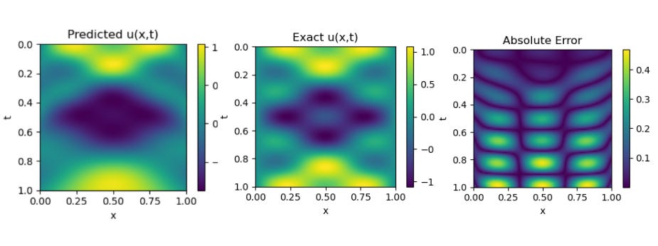
1D Wave Equation

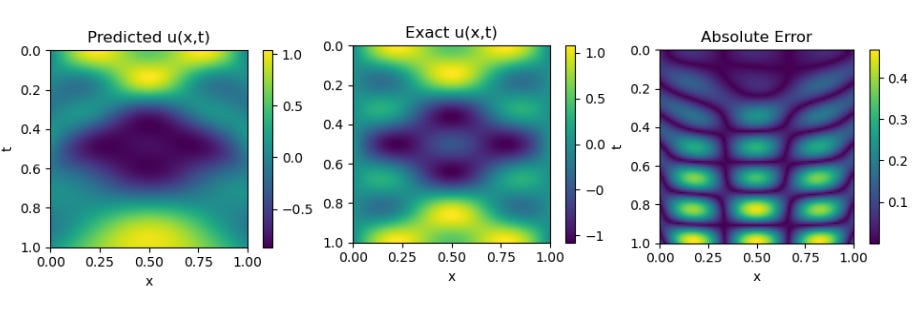
Results obtained by Implementing PINNsformer with default Hyperparameters desrcibed in paper We can observe that, for the 1D Wave Equation, additional hyperparameter tuning is required. In the lower region of the plot, the predicted solution does not perfectly align with the exact one the predictions appear slightly diluted. In contrast, the results shown by the authors in their paper exhibit a much closer match, indicating that further optimization of parameters could help bridge this gap in our implementation.

Results from PINNsformer Paper , Source :- https://github.com/AdityaLab/pinnsformer Navier Stokes Equation

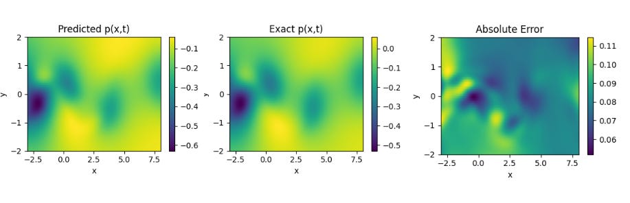
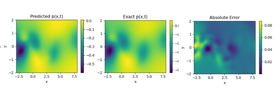
Results obtained by Implementing PINNsformer with default Hyperparameters desrcibed in paper on Navier Stokes Equation. 
Results from PINNsformer Paper , Source :- https://github.com/AdityaLab/pinnsformer We can see that the model predicts the solutions of the standard PDEs with high accuracy and relatively low error across all three cases. These results highlight the strong generalization capability of the PINNsFormer architecture. We are currently extending our experiments to explore its performance on other classes of equations to further evaluate its robustness and adaptability.
6. Why PINNsFormer Beats Classical PINNs
Classical MLP-based PINNs are effective for solving PDEs but face key limitations in handling temporal dependencies, maintaining smooth convergence, and generalizing to complex physical systems. They treat inputs as static, pointwise data and often rely on non-smooth activations such as ReLU or tanh, which can cause unstable gradients and irregular loss landscapes. As a result, classical PINNs frequently struggle with convergence and exhibit limited generalization beyond simple, low-dimensional problems.
PINNsFormer overcomes these challenges through a Transformer-based architecture and wavelet-inspired activations. By capturing causal temporal relationships and leveraging multi-head attention, it learns both global and local dependencies across space and time. The smooth, Fourier-like wavelet activation stabilizes gradients, leading to faster and more consistent convergence. Overall, PINNsFormer generalizes better, converges more reliably, and models real-world physical dynamics with higher accuracy and stability than traditional PINNs.
7. Broader Implications
The innovations in PINNsFormer extend far beyond PDE solving:
Wavelet activations could serve as drop-in replacements for standard activations in Transformers, GNNs, and implicit neural representations.
The pseudo-sequence framework opens doors to learning causal relationships in scientific time-series, fluid dynamics, and multi-physics simulations.
Integrating PINNsFormer with Neural Tangent Kernel (NTK) theory, adaptive sampling, or meta-learning can yield hybrid models capable of addressing high-dimensional, multi-scale PDEs.
In essence, PINNsFormer stands as a step toward the fusion of symbolic physics and attention-based deep learning, reshaping how we model the real world.
8. Summary
PINNsFormer is not just an incremental upgrade over classical PINNs it’s a reimagining of physics-informed learning through the lens of transformer-based attention and spectral activations.
It signifies a broader trend in Scientific Machine Learning (SciML): bridging rigorous physics with flexible neural architectures.
As the boundaries between numerical methods and neural computation blur, architectures like PINNsFormer pave the way toward universal differentiable solvers that can learn, reason, and generalize across scientific domains.
I have curated detailed video on how I have implemented PINNsformer and explained all the concepts in detail. Please have a look and let me know if you have any Questions.