How does ACT (Action Chunking with Transformers) actually work?

Jan 10, 2026

The ACT architecture was first described in a paper which came out in 2023:

Why did it gain attention?

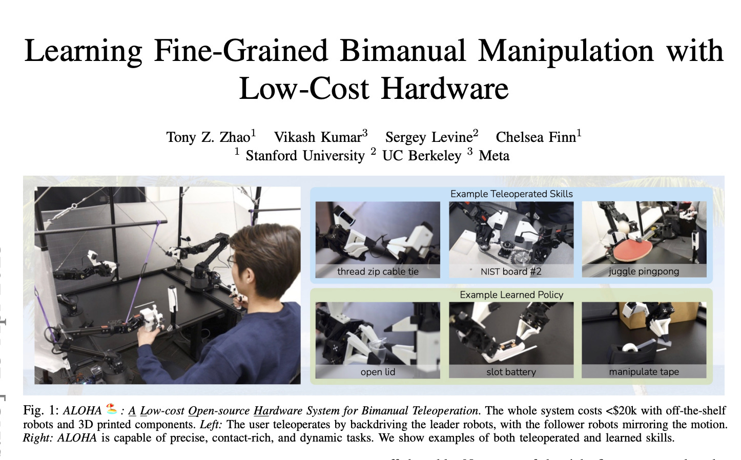
This paper showed that for the first time, AI policies can be implemented in low-cost hardware for achieving complex tasks.

Some tasks which were completed using the ACT policy included:

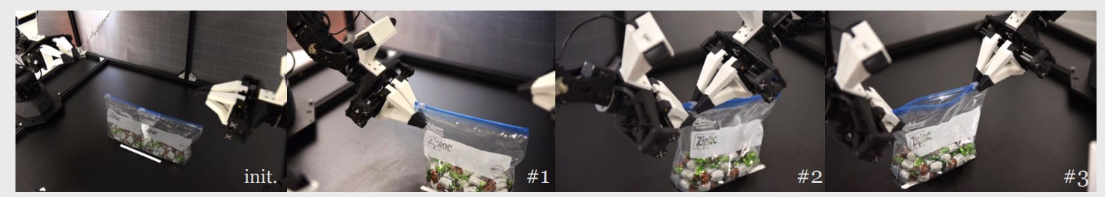
(1) Opening a ZipLoc bag:

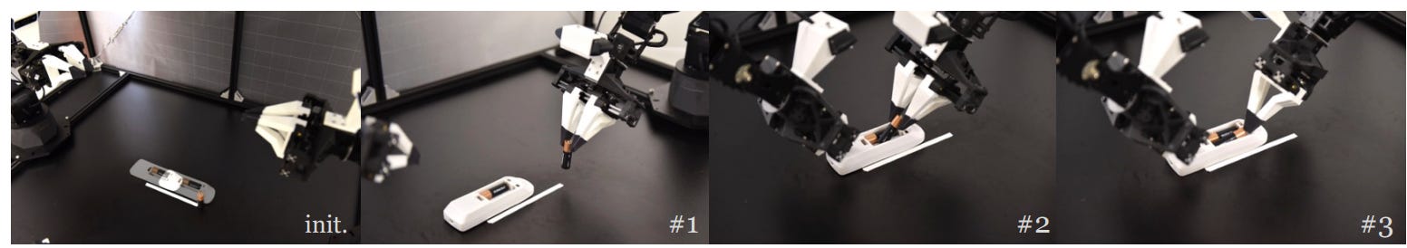
(2) Slot Battery:

(3) Open Cup:

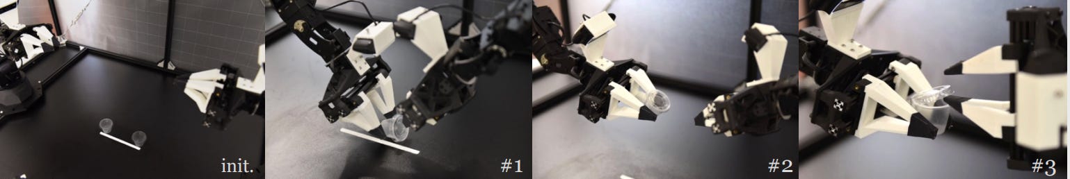
All of these are tasks which require fine manipulation.

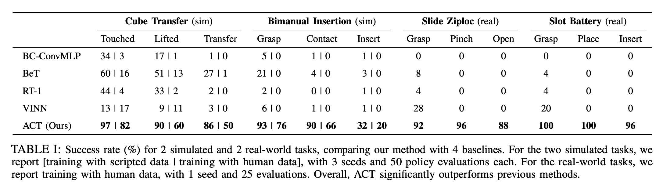
Have a look at the gains the policy achieved compared to other policies! Naturally, it caught attention of the Robotics community.

There are innovations in both the hardware and the software side. An example of low-cost hardware, where ACT can be successfully implemented in the SO-101 Robot (a practical on this is coming soon!)

Hugging Face Launches the SO-101, an Upgraded Low-Cost 3D-Printable Autonomous Robot Arm - Hackster.io

In this article, we are going to focus on the software side of the innovation.

Once you read the paper, you realize that there are 3 things on the software side which make this policy unique:

(1) It used a Conditional Variational AutoEncoder

(2) It uses a DETR-inspired Transformer Decoder

(3) It uses Action Chunking

Don’t worry if these words sound a bit complex, we are going to go over everything in detail!

We will cover the architecture of the ACT policy in a series of Architecture Versions, where we will think from first principles and understand how the architecture evolves.

First, let us understand what we want to do:

We want to predict the distribution of the variation of the joint angles, given the state of the robot.

Architecture Version 0:

So, our first thought is that, we need the following:

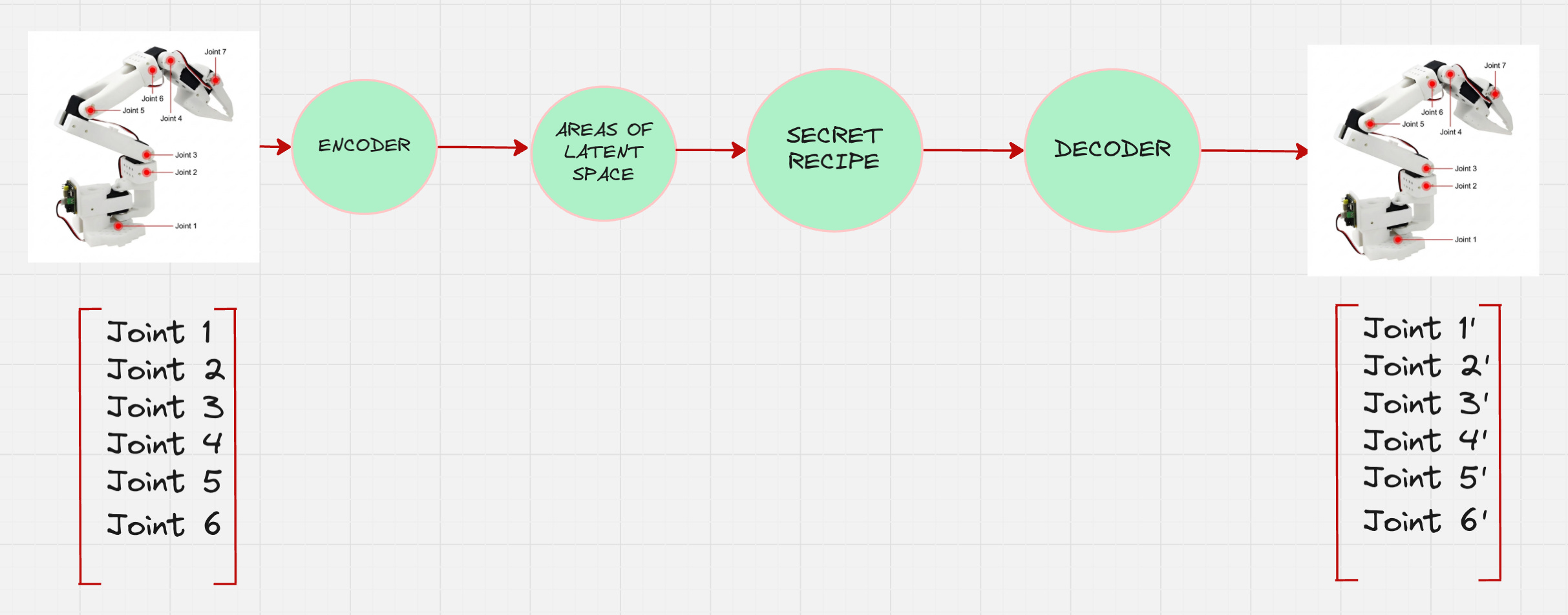
Have a look at our article on Variational AutoEncoders here to understand the above diagram properly: https://vizuara.substack.com/p/variational-autoencoders-explained

This is a great start, but we can immediately see there is one major drawback of this approach.

Even if we manage to train this Variation AutoEncoder, at the end of it, we will get different actions which are the joint configurations sampled from the action space. So, the robot will move randomly.

We do not want that. We want the robot to move in a specific way for a specific robot configuration.

Architecture Version 1:

We want to model the distribution of the joints given the current state of the robot.

This is how we will modify our architecture:

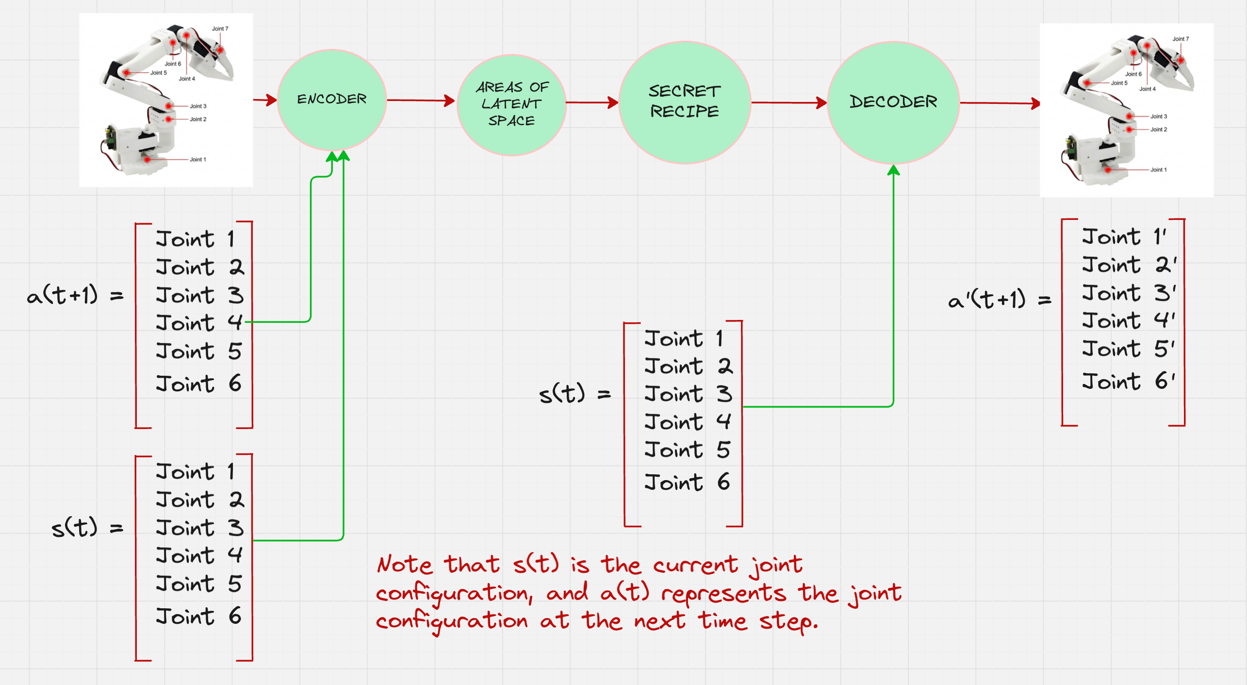
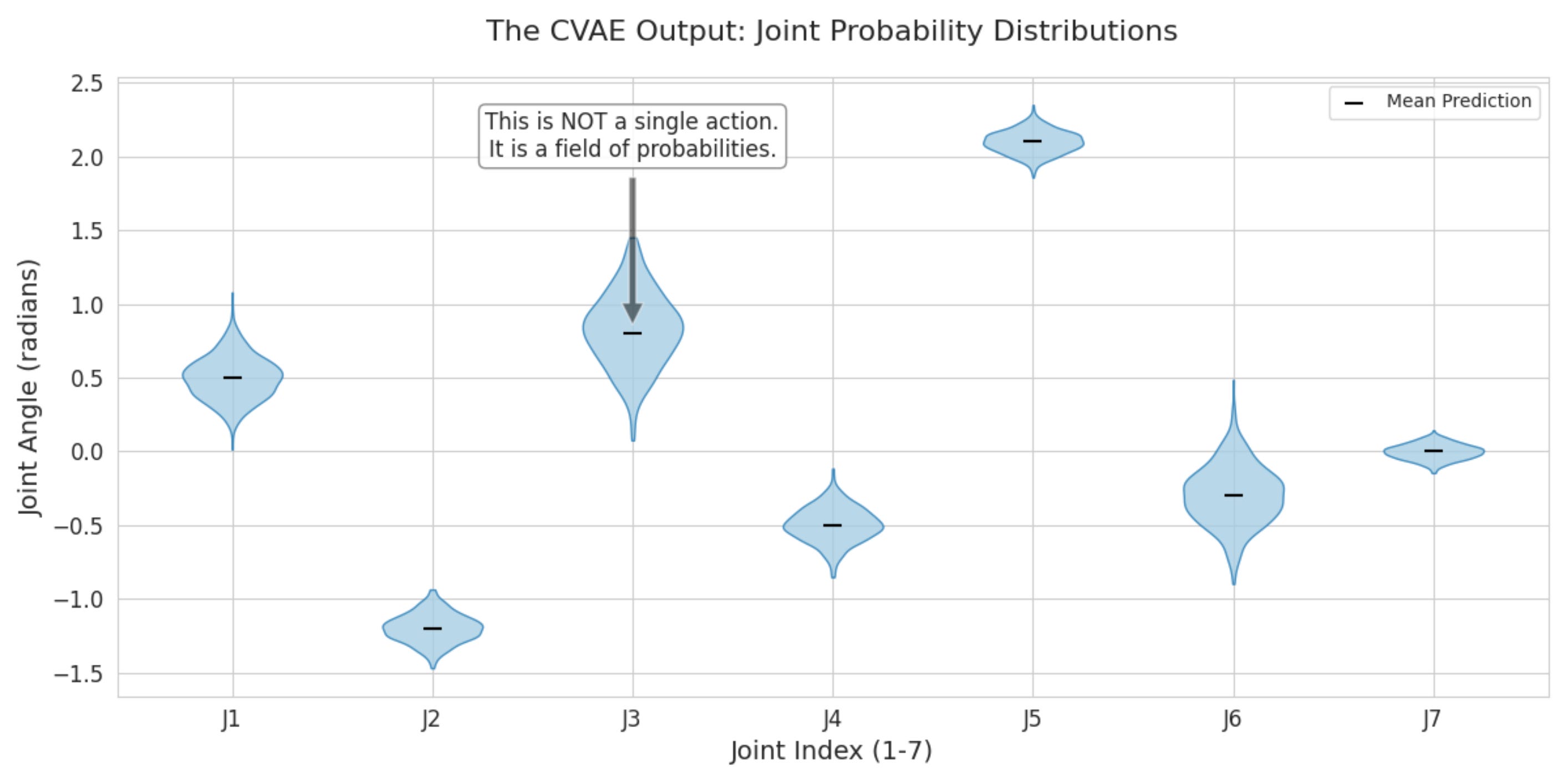
This looks like a decent setup. Just so that we can be clear, the following diagram visually represents the distribution that we are trying to predict.

There is another crucial point which comes to mind at this stage.

Don’t you think that the distribution of the joint angles not only depends on the current state of the robot but also the environment around it?

For example, if the task of the robot is to pick and place an object, then the distributions will greatly change if the robot is close to the object or not.

Architecture Version 2:

The environment around the robot is captured with the help of cameras. So we have images which are obtained from by these cameras.

So the final architecture that we are thinking about looks as follows:

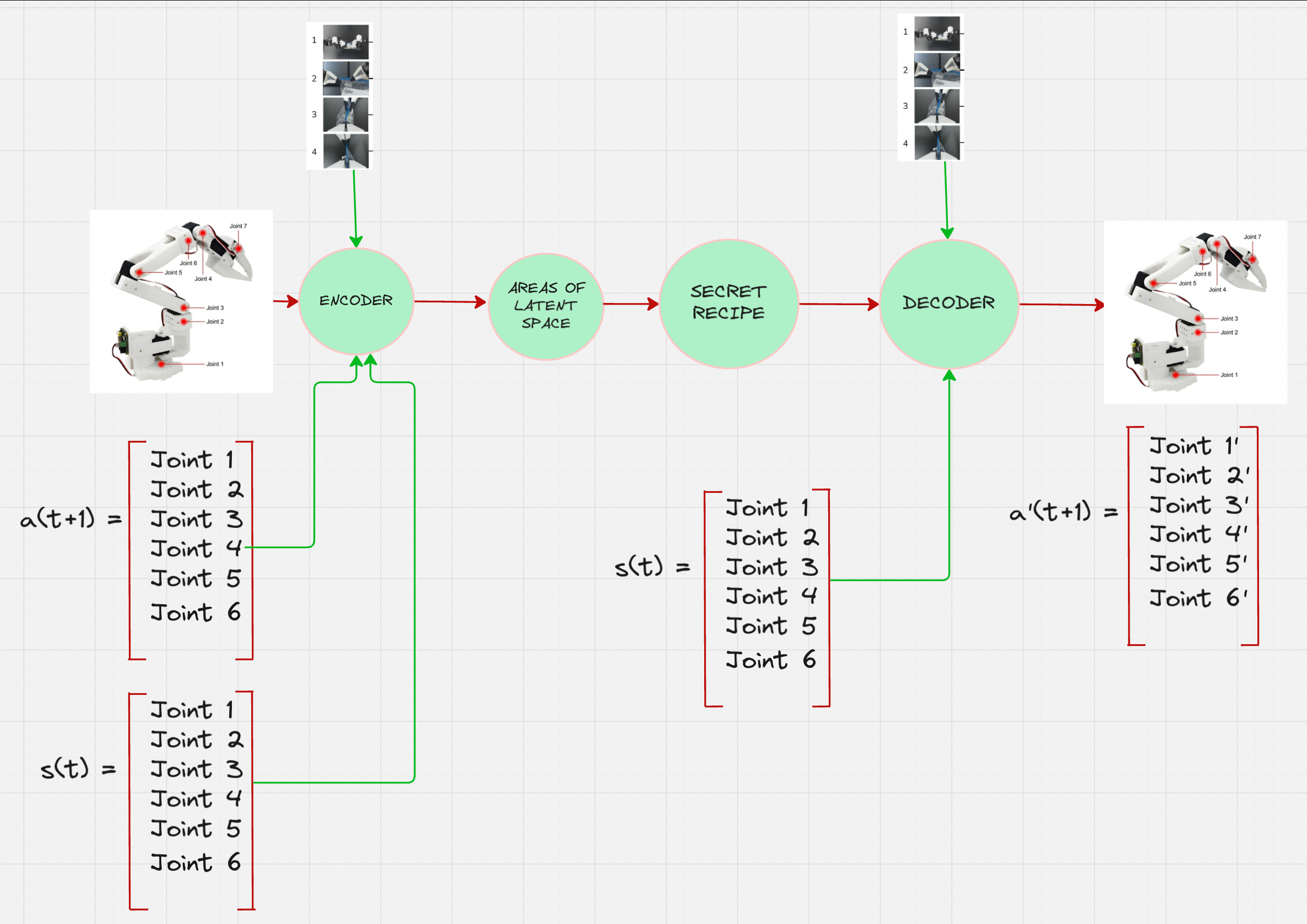
We are trying to predict the variations in the joint angles conditioned on the position of the joints as well as the images collected from the camera feeds.

This architecture is also called a Conditional Variational Autoencoder.

Now, let us understand the encoder and the decoder separately.

First, we start with the encoder.

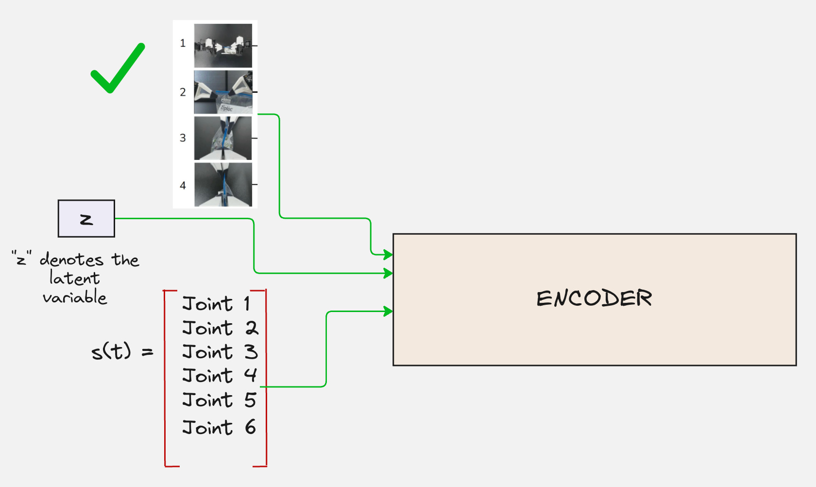
Let us start with what first comes to our mind regarding the encoder architecture.

The following is the first architecture that comes to my mind:

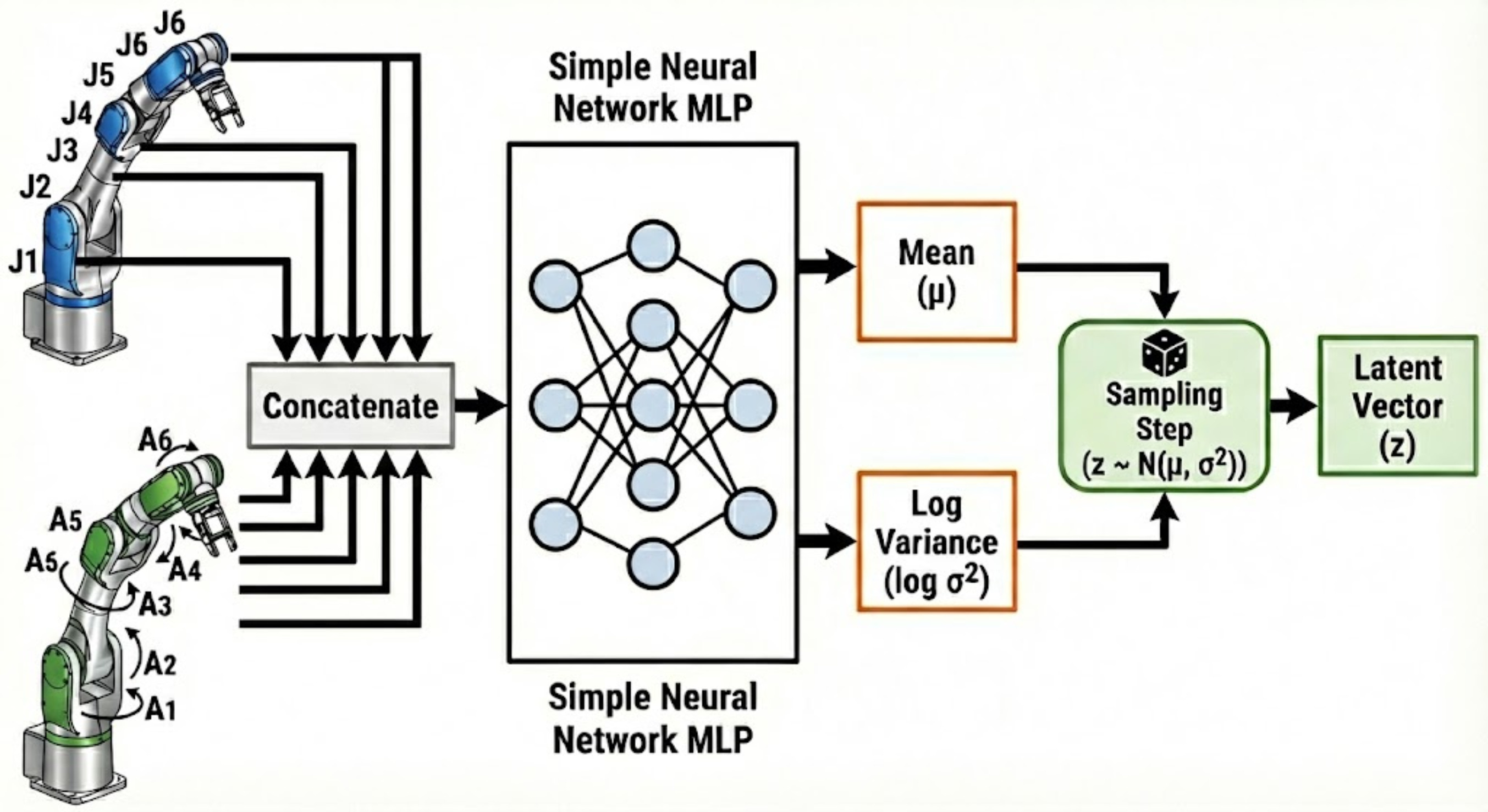
Note that here we have conveniently ignored the input images from the camera feed.

This is a great start, but this is not the architecture which is used in the ACT paper.

The main reason is that in the ACT paper, they do not consider one single action, rather they consider a sequence of actions for a given state.

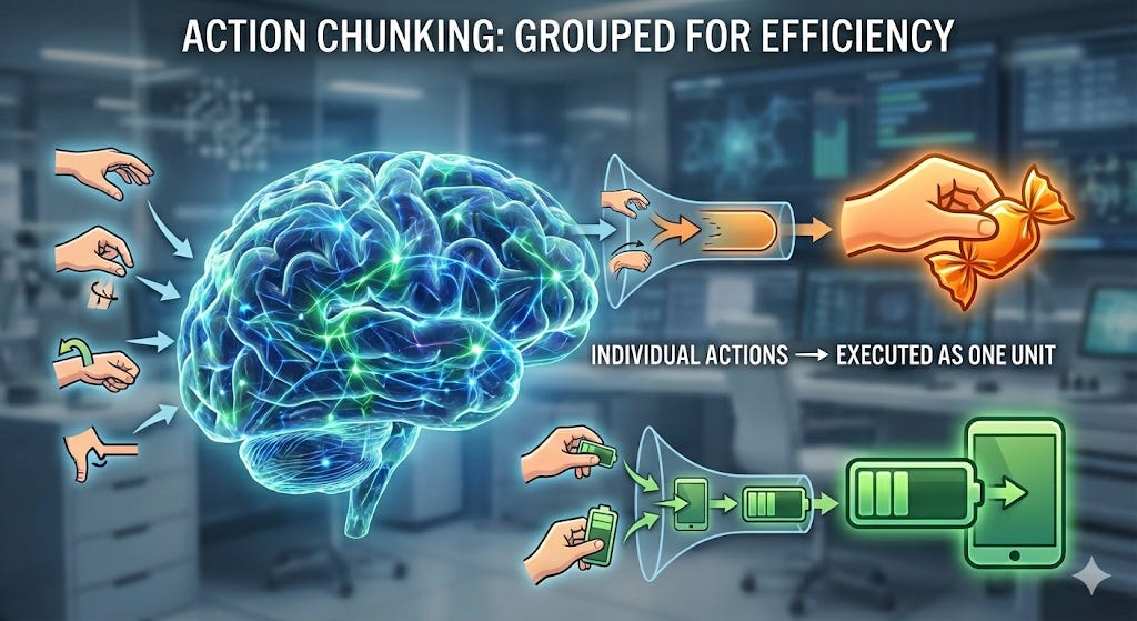
The process of predicting a sequence of actions instead of one is called chunking.

This is inspired by a neuroscience concept where individual actions are grouped together and executed as one unit, making them more efficient to store and execute.

Intuitively, a chunk of actions could correspond to grasping a corner of the candy wrapper or inserting a battery into the slot.

This means that the encoder pipeline looks something as follows:

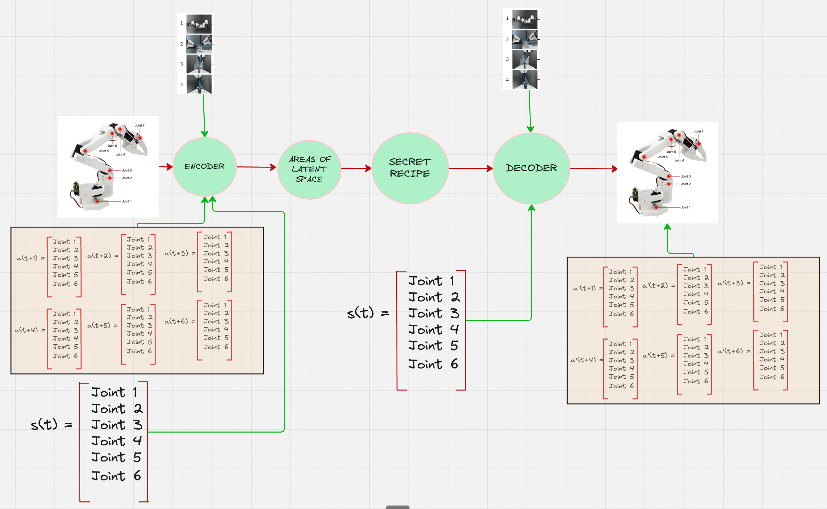
Architecture Version 3:

How an MLP sees it: An MLP sees the whole sequence as one giant, flat bag of numbers. It doesn’t inherently understand that Action 1 comes before Action 2. It has to learn these relationships from scratch using brute force (massive amounts of data and weights).

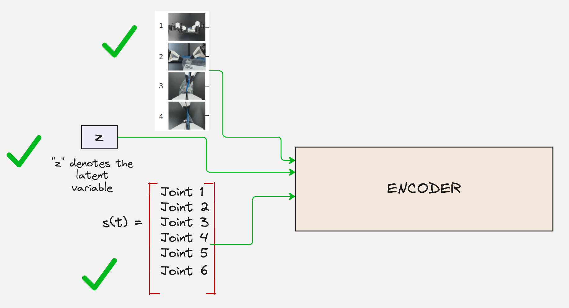
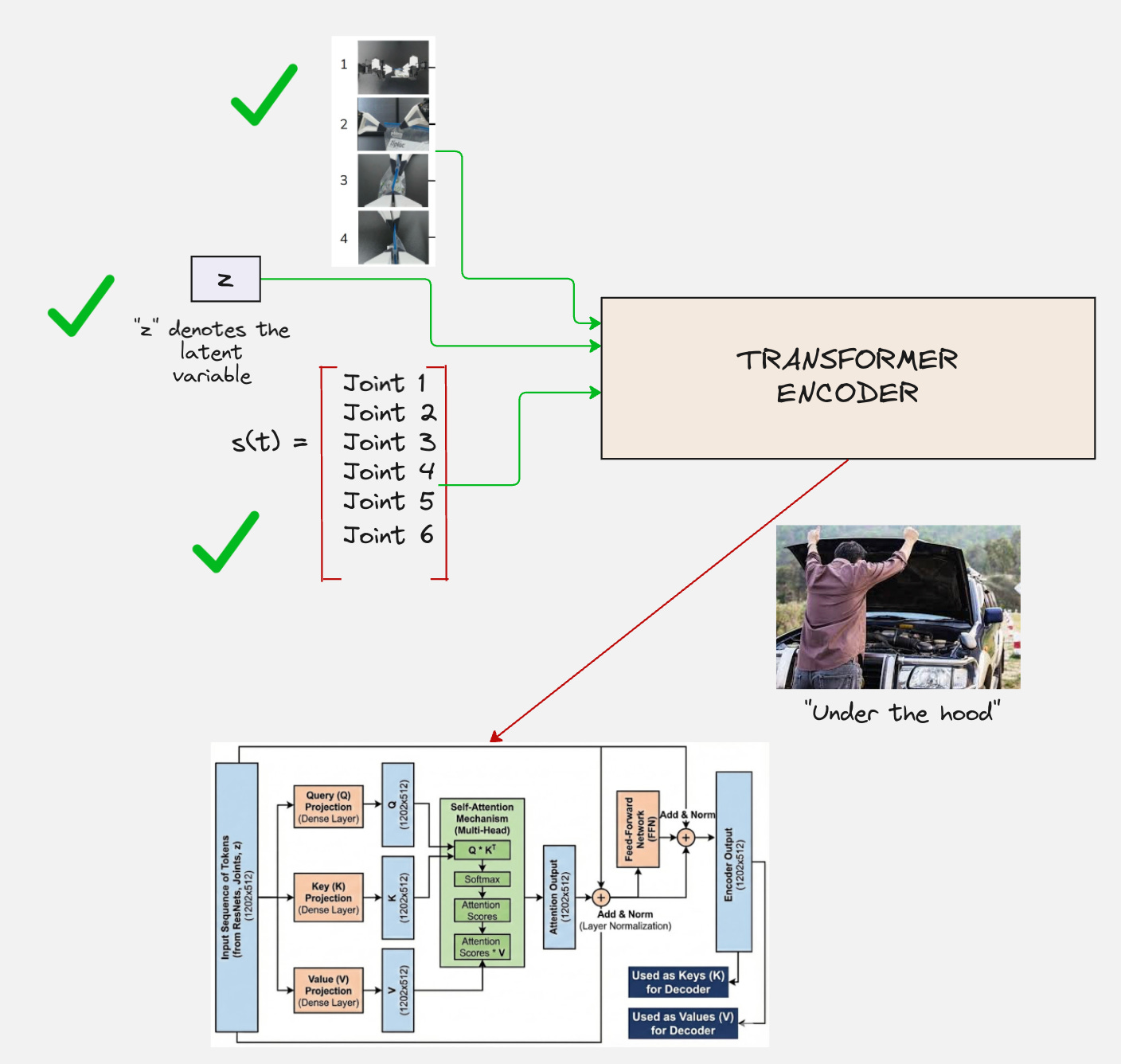
Hence we don’t use a multi-layer perceptron. Instead, we use a transformer encoder.

So, broadly speaking, our encoder-architecture looks as follows:

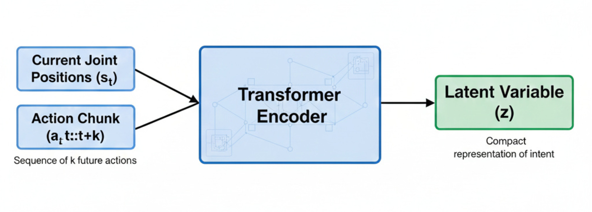
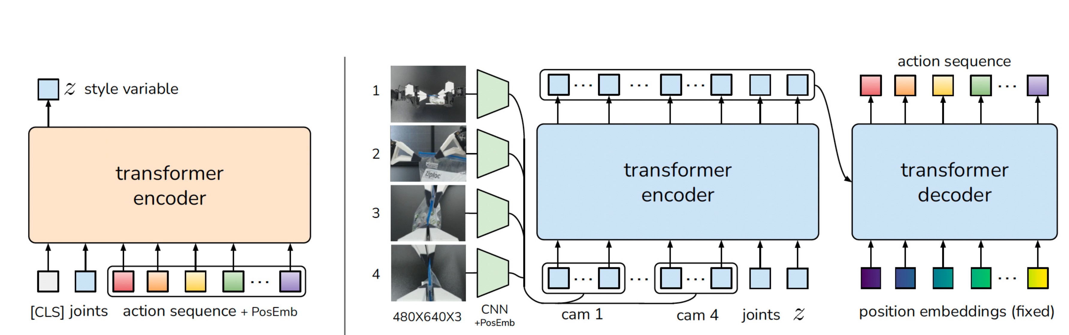
The transformer encoder has the following architecture:

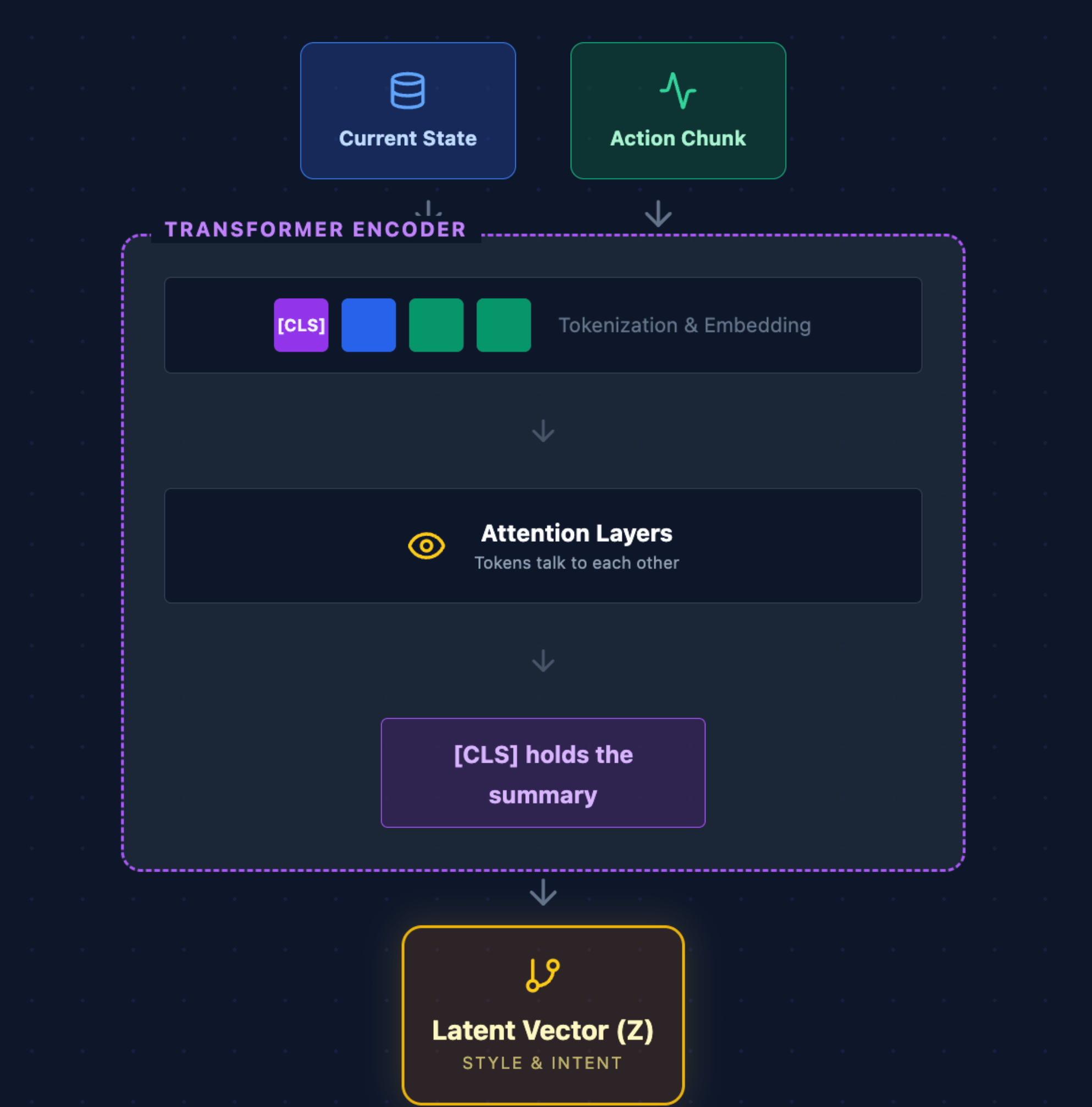
First, the current state and the action chunk are tokenized. In this process, embedding vectors are created for each state and action vector.

These embedding vectors are then passed to the subsequent layers.

The most important layer is the attention layer, which understands the relationship between each token and generates attention scores for each pair of tokens.

These attention scores are then used to modify the values of the embedding vectors.

To generate the latent vector, all we need to focus on is the CLS token and the values which are present inside the CLS token.

Let us look at an interactive visualization to understand all the steps in detail:

https://actencoder.vizuara.ai/

Now that we have understood how the encoder looks like, let us understand numerically what happens to the tokens as they pass through the encoder.

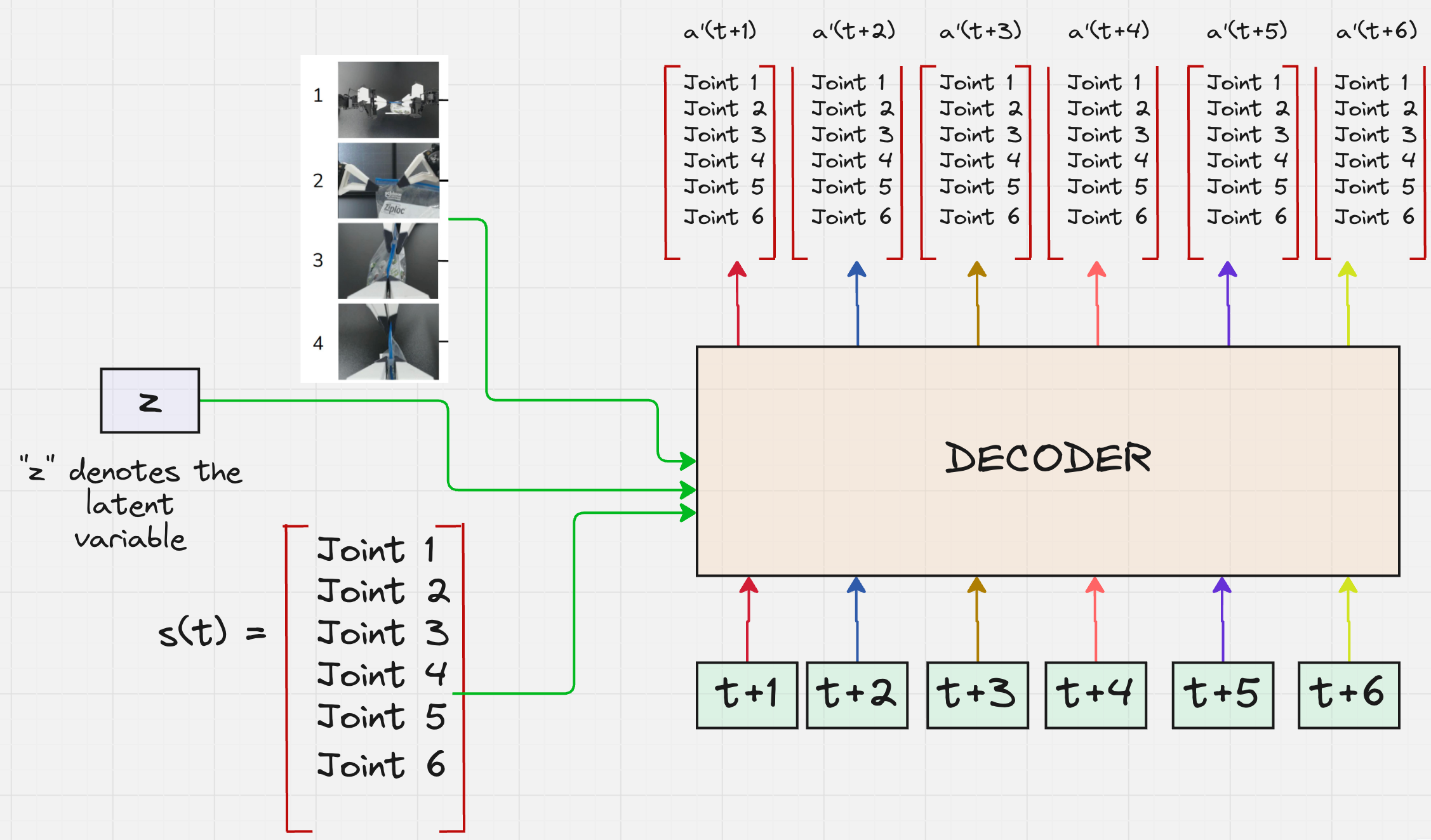
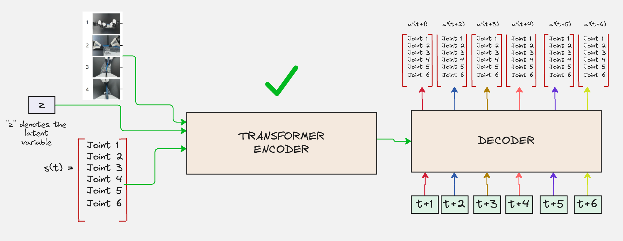
ACT Decoder

We want our ACT decoder to do something like this:

You might realize that there is a problem with the above architecture.

Architecture Version 4:

To understand the next time steps for the robotic joints, we need the current joint positions and the inputs from the camera feeds as well.

The modified architecture looks as follows:

Let us imagine a scenario, where a robot arm is positioned to pour coffee, with visual representations of both an overhead camera view and a wrist-mounted camera view.

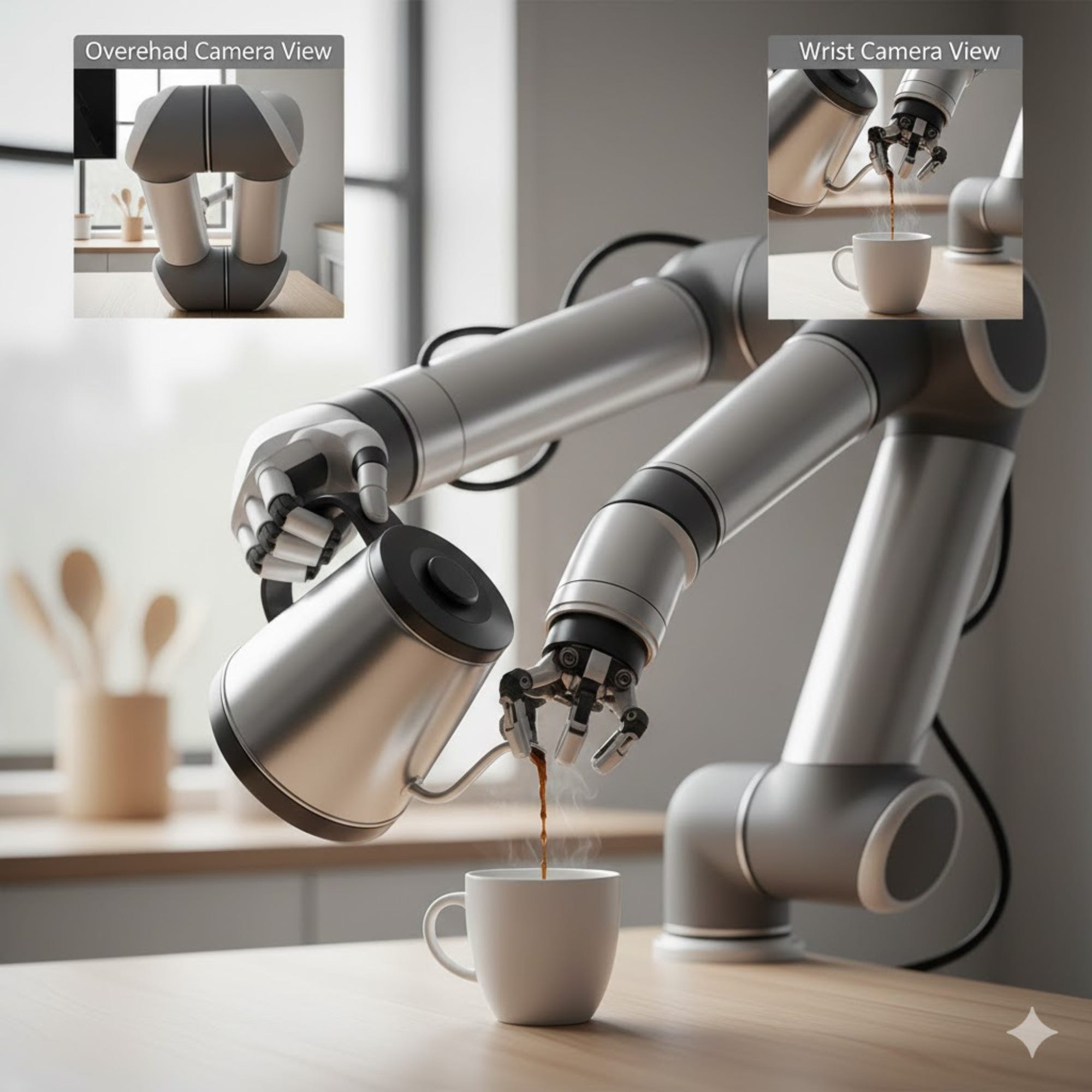
The robot has two eyes:

(1) Overhead Camera: Looks down at the table.

(2) Wrist Camera: Mounted on the robot’s hand, looking closely at the gripper.

Now consider the following situation: The robot is about to pour its arm moves over the mug:

The Overhead Camera is now blocked by the robot’s own arm (it can’t see the mug anymore).

The Wrist Camera is the only one that can see the mug now.

To understand where the mug is in 3D space, the robot needs to combine the information from both cameras instantly.

This is not happening in the above architecture!

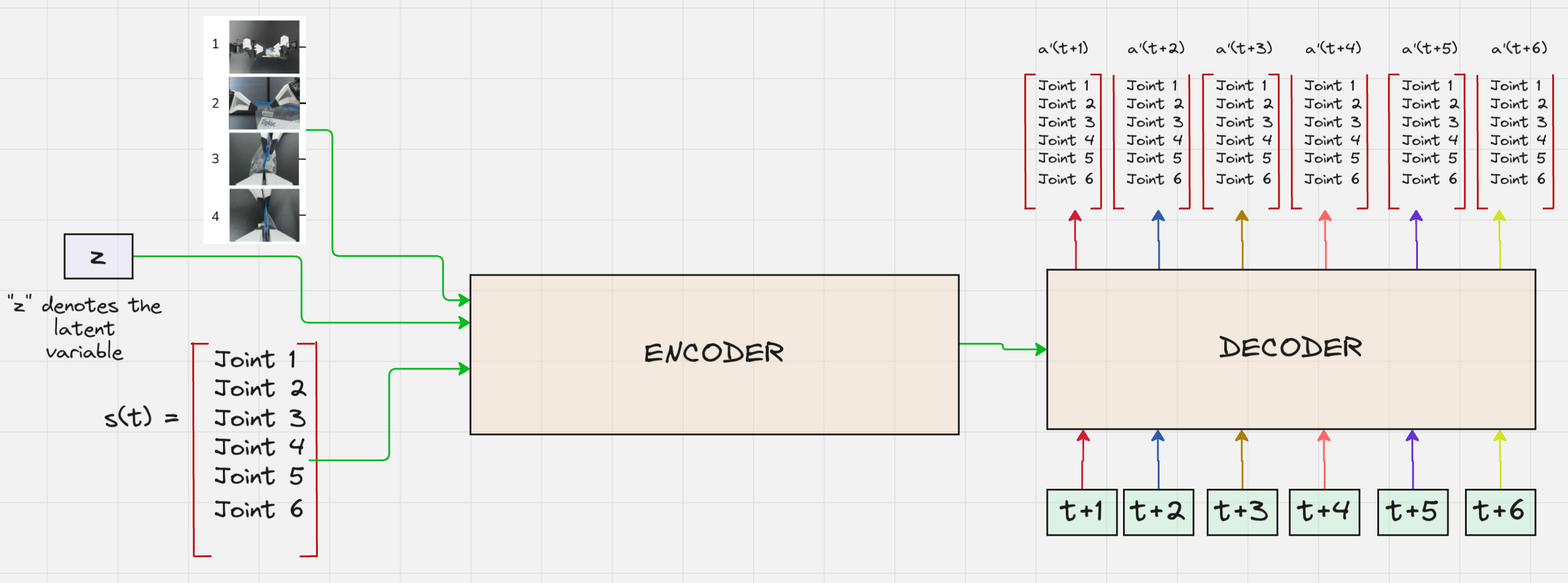
Architecture Version 5:

This fusing of information is exactly what an encoder does.

So now we can modify the architecture of the decoder as follows:

First, let us understand how the fusing of this information happens, which is passed as an input to the encoder.

Let us start by focusing on the images.

Let us consider that the robot is pouring coffee from a mug. Here are the four images collected from the four cameras:

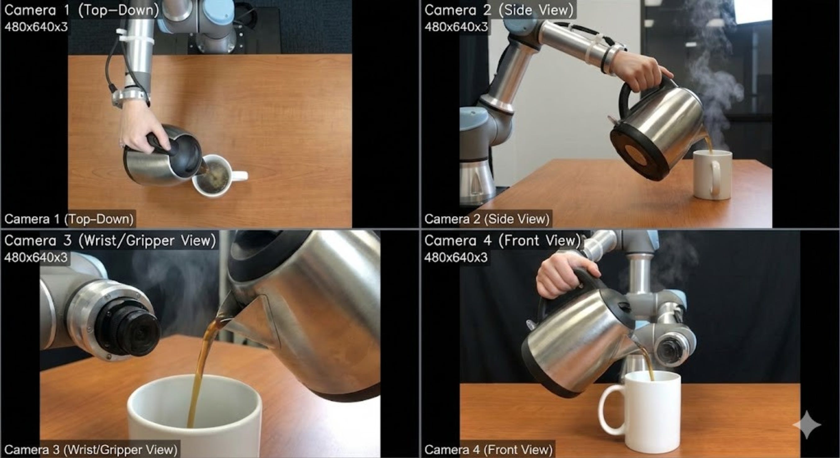
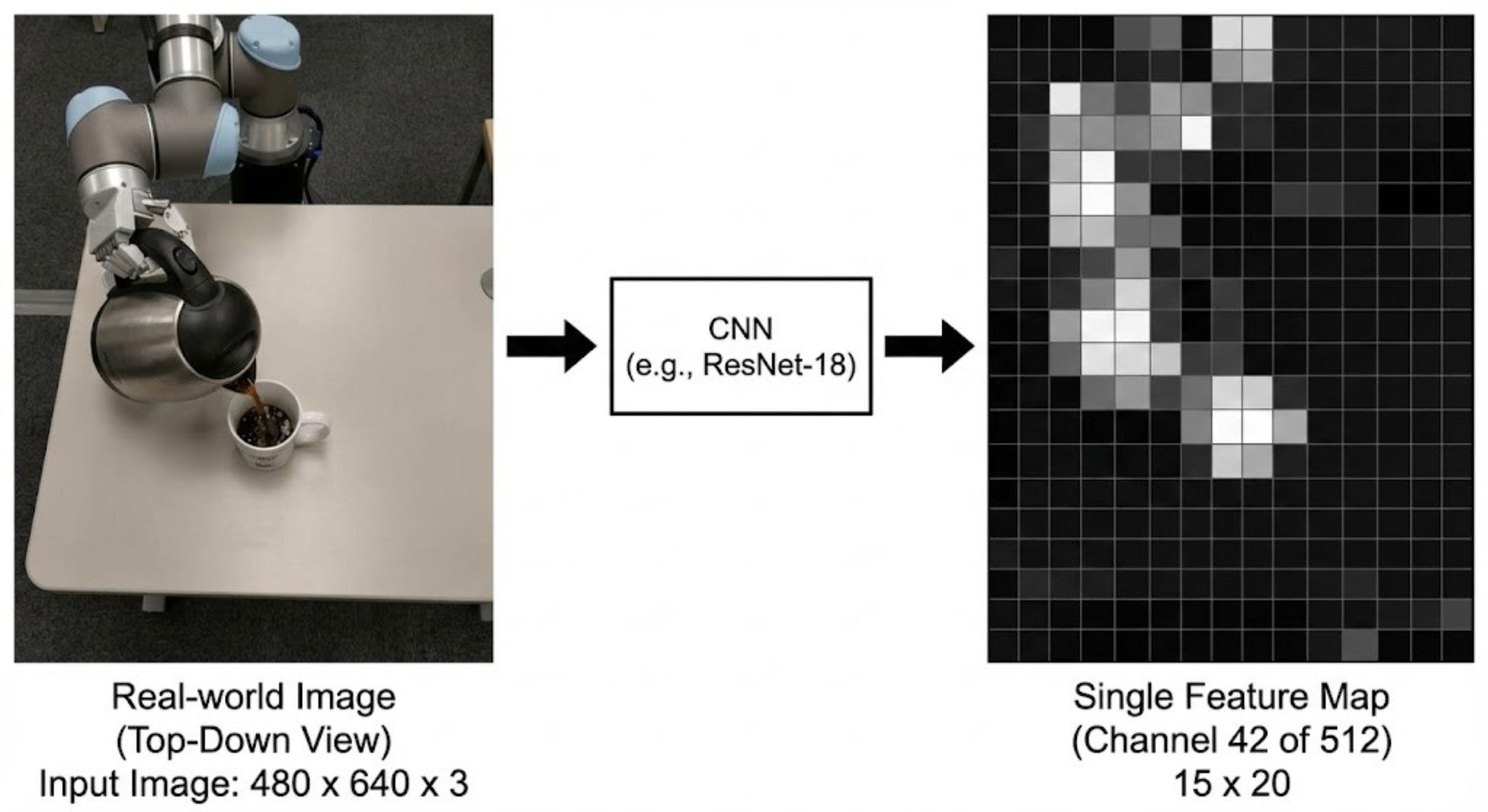
These 4 images are then passed through a CNN, which reduces the spatial dimension of the image to 15x20 and increases the depth to 512 dimensions.

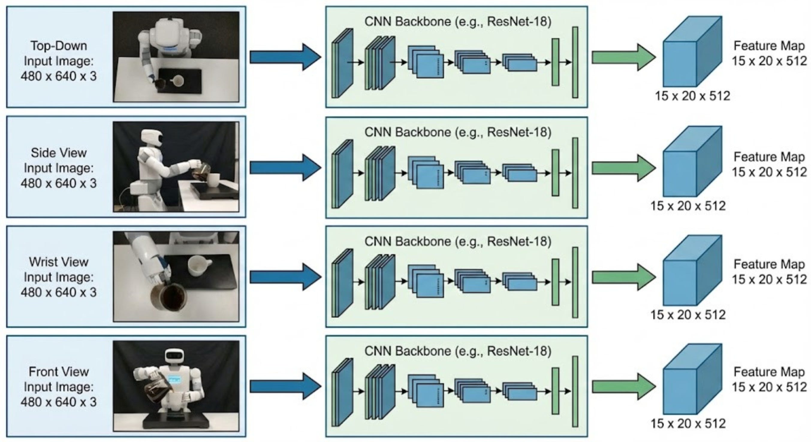
An example feature map can look as follows:

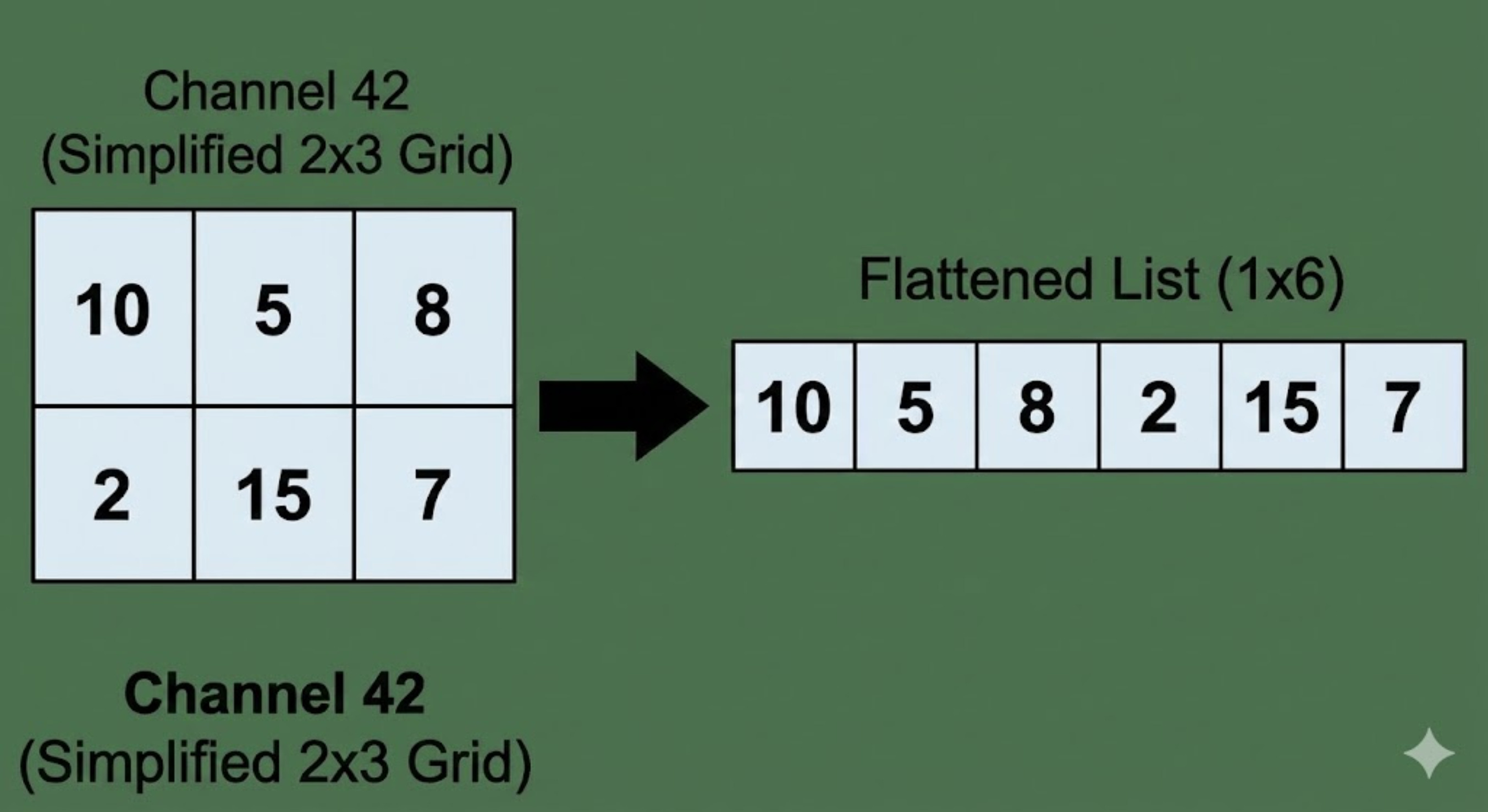
Next, we convert these feature maps into one single list. For that, we need to flatten the 15x20 vector into a single vector of 300 dimensions.

The flattening process looks like this. Imagine the same transformation happening for the size of 15x20.

So, our architecture is modified to look as follows:

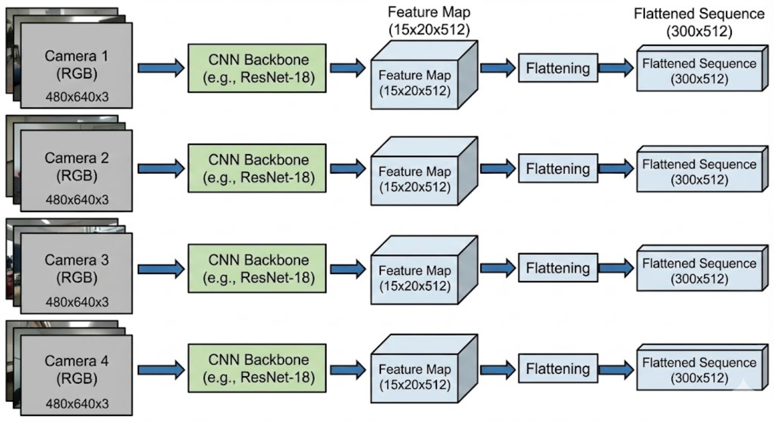
So, totally 1200 vectors with dimensions 512 are passed to the encoder.

Let us move on to understanding how the inputs for the joint positions are created.

We use a linear layer for this purpose:

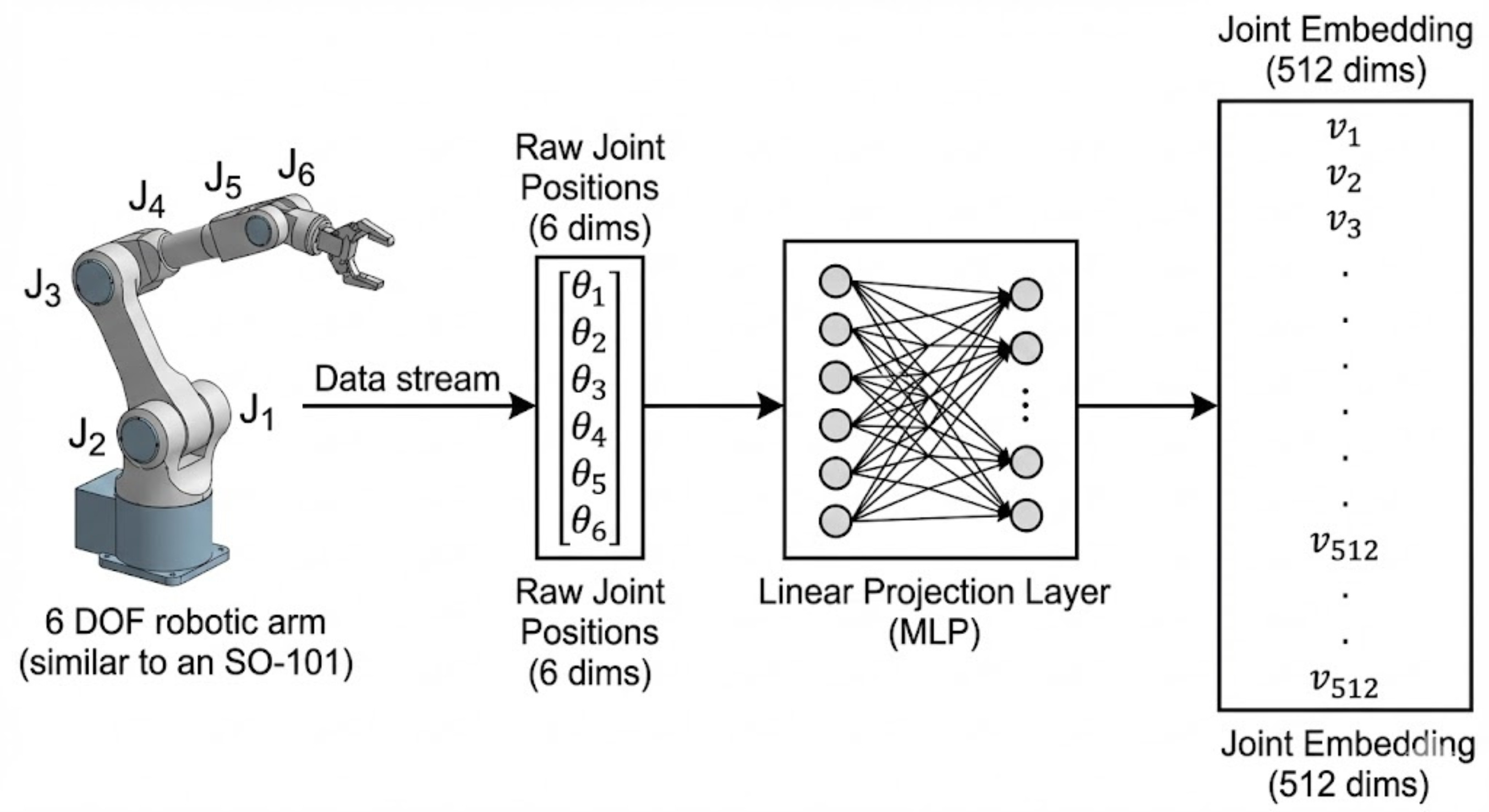
This completes the processing of the inputs which are passed to the encoder.

What about the encoder?

As discussed before, we need the encoder because it has to synthesize all three different types of data:

Visual Data (High dimensional): Pixels/Features from 4 cameras.

Proprioceptive Data (Low dimensional): Precise numbers for joint angles.

Latent Style (z): A abstract “instruction” on how to behave (e.g., “move fast”).

Now, all these data types are very different, and if we just stack them side-by-side, the model wouldn’t know how they relate.

So, we need some mechanism to force these modalities to talk with each other.

Example: It links the “Gripper Token” (from Joint data) with the “Mug Handle Token” (from Camera 1).

Result: It creates a new understanding: “The gripper is currently 2cm away from the handle.”

This is exactly what the self-attention mechanism in the transformer architecture does. Hence, we use a transformer encoder for this.

Architecture Version 6:

Have a look at the visualization below to understand this in detail:

Now let us look at our original architecture for the ACT decoder.

Now let us look at the Decoder:

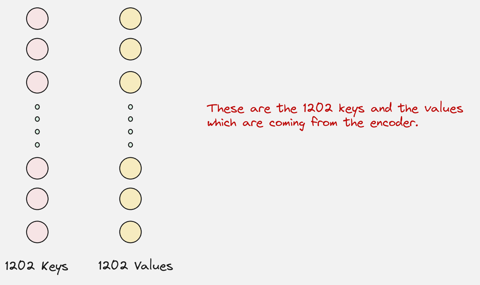
But what about the keys and values?

Let us revisit the encoder architecture again:

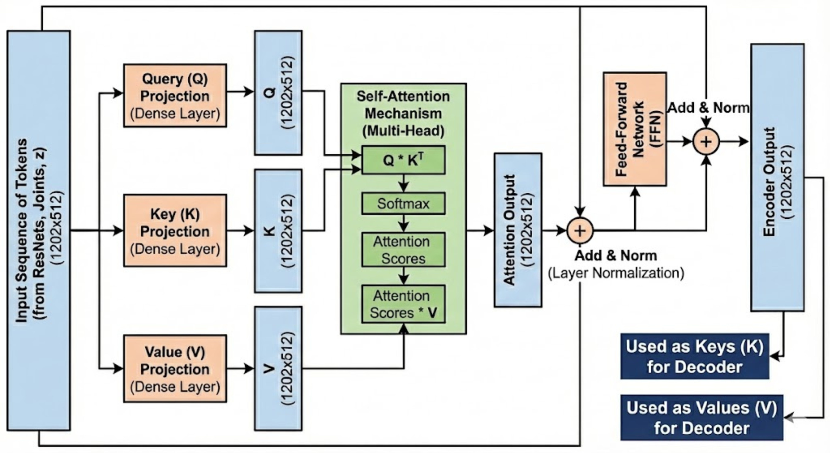
Here, we can clearly see that the output of the encoder is the keys and the values which will be used by the decoder.

Now, we will perform the cross-attention.

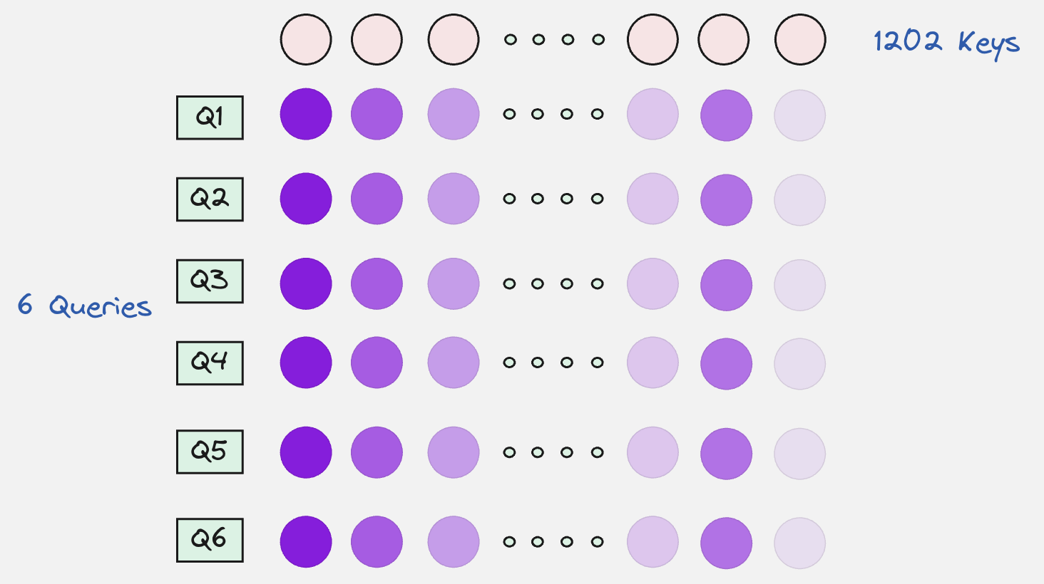
Once we calculate the attention scores, we will use the values to compute the context vectors.

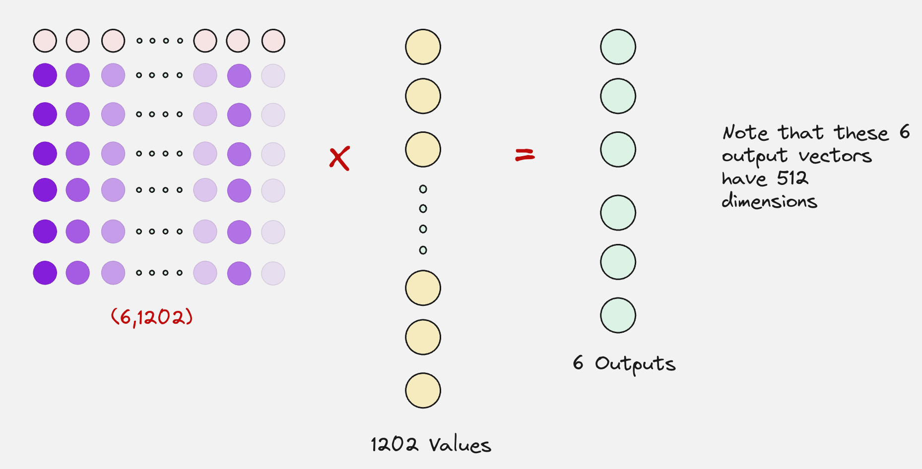
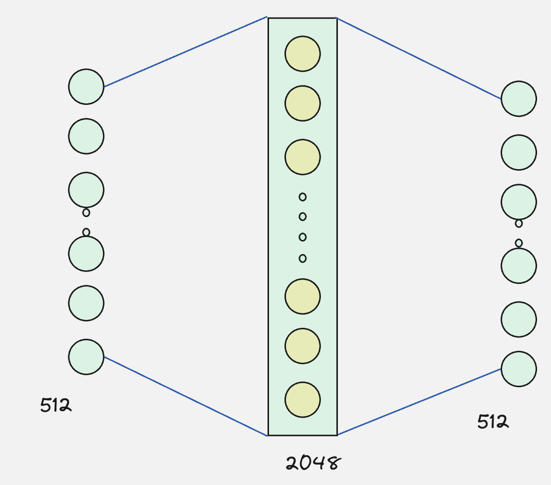
These context vectors will now be updated by passing them through an MLP layer:

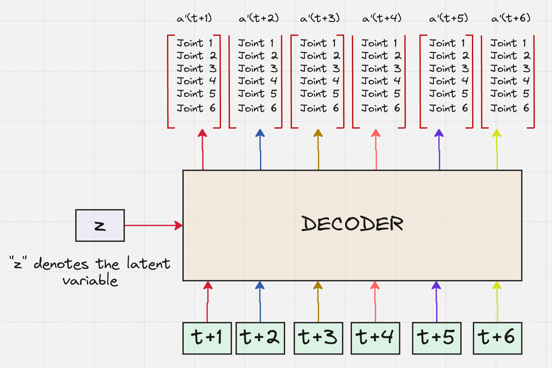
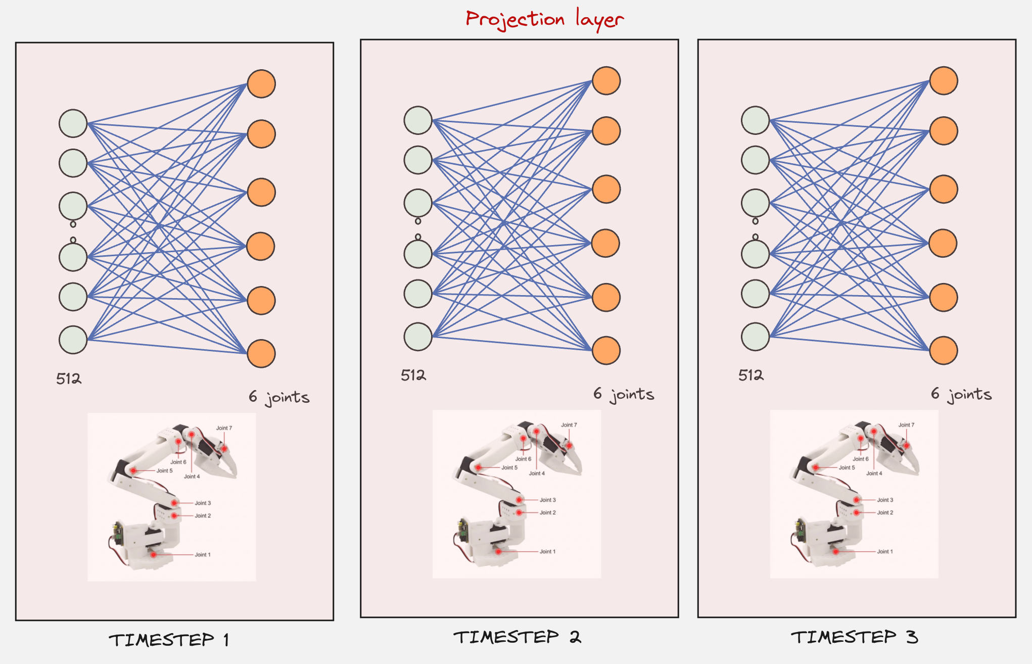
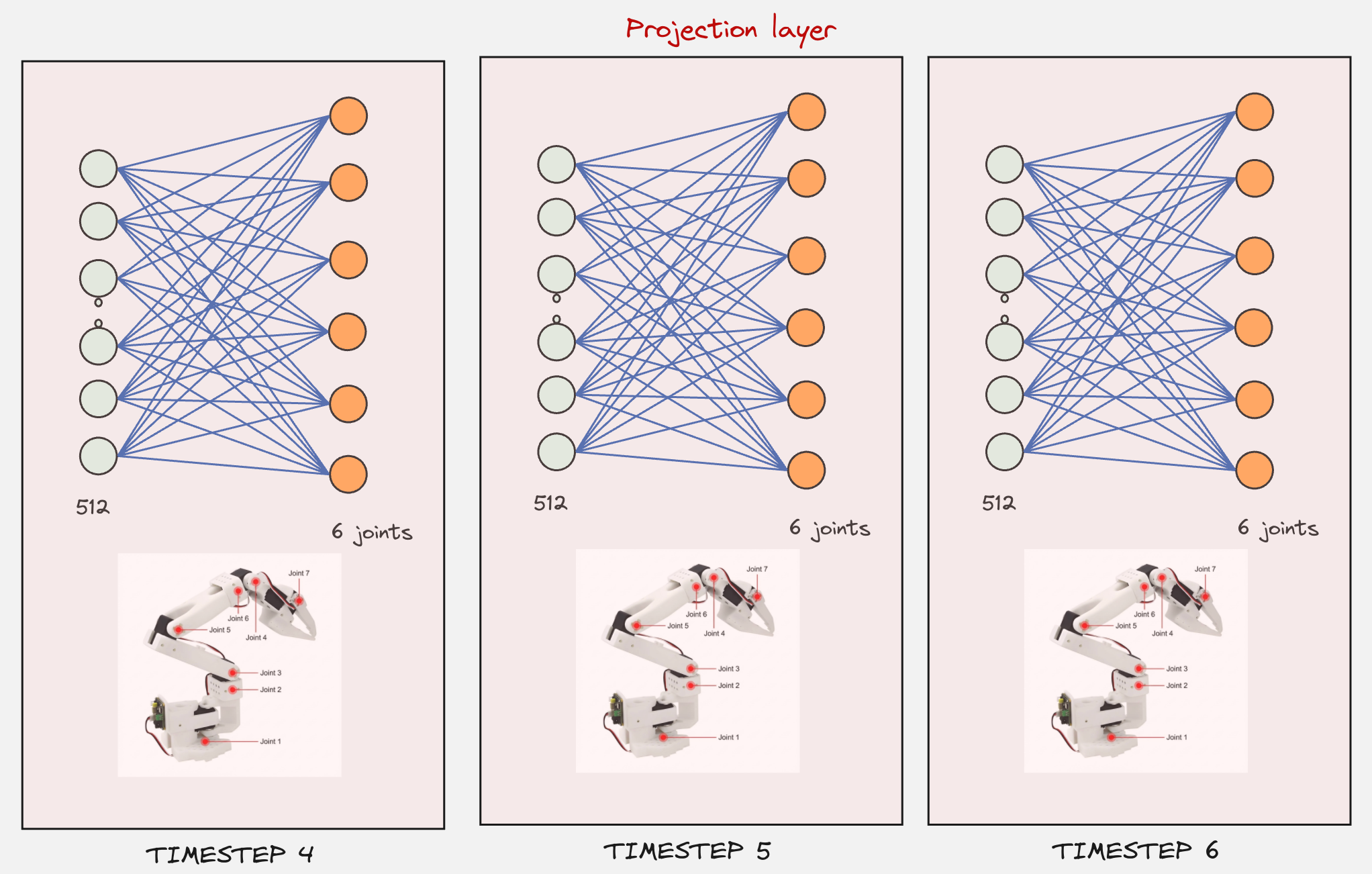
In the final step, this will be passed through a projection layer, where the 512 values will be converted to the 6 joint values. This will happen for the number of timesteps included in the action chunk (e.g: 6).

Now, let us piece all of this together and see how the final architecture for the ACT Variational AutoEncoder looks like:

How is the Decoder similar to DETR?

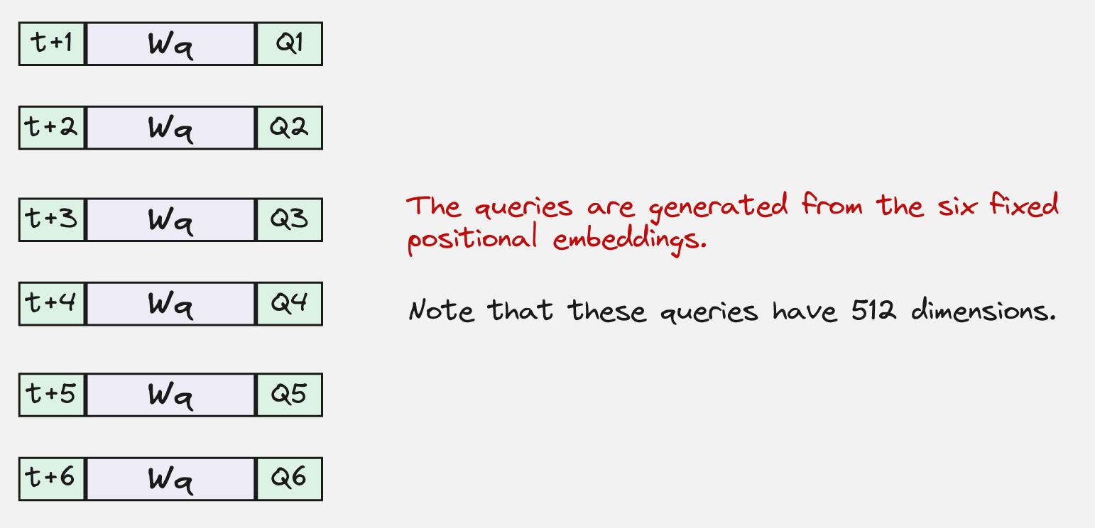
In a standard setup, the inputs at the base of the decoder are word-token embeddings corresponding to the text the transformer is trained to generate.

By analogy with the original transformer architecture, one option would be to feed in a start-of-sequence token followed by embeddings of the actions to be predicted, effectively casting the task as next-action prediction.

However, this formulation comes with a key constraint: it requires causal attention. As a result, when predicting the action at time t, the model can only attend to actions up to t–1.

To avoid this limitation, the authors take a clever alternative route by borrowing ideas from DETR (DEtection TRansformer). This design allows the decoder to reason over the entire output sequence at once, free from the restrictions imposed by causal masking.

Have at look at this video, which talks about the intuition behind DETR:

During training, both the transformer encoder and decoder networks are trained. However, during testing, we discard the encoder and only use the transformer decoder.

The value of the latent variable (z) is set to 0 during inference, for deterministic trajectories.

It’s like telling the encoder–decoder transformer at inference time: you’ve already learned from a vast range of trajectories—now just focus on taking me from point A to point B. The uniqueness of the path no longer matters.

The training loop for the ACT Policy looks as follows: