How AlexNet changed the trajectory of Computer Vision

And how we tried to recreate that magic with five flowers and a coffee cup

and

May 11, 2025

In 2012, a seismic shift occurred in AI. A model named AlexNet bulldozed through the ImageNet competition, leaving every other approach in the dust. It did not just win - it changed the rules of the game.

Before AlexNet, image classification was a painstaking affair involving handcrafted features, edge detectors, and a lot of mathematical duct tape. Think SIFT, HOG, color histograms, and hours spent tweaking filters to "find the cat."

Then came AlexNet - with 60 million parameters, 5 convolution layers, 3 fully connected layers, and a GPU-powered training process - and said: Let the model learn the features itself. Also, please stop using CPUs.

The rest is history.

What made AlexNet special?

Let us break down what made AlexNet not just good, but revolutionary:

Convolutional layers that learned filters directly from data
ReLU activation, which made training faster and reduced vanishing gradients
Dropout for regularization, reducing overfitting
Max pooling to downsample without losing key features
And crucially, GPU training that made all of the above practical at scale

It was trained on 1.2 million images from ImageNet across 1,000 categories. At the time, this scale was unheard of.

But here is the kicker: AlexNet beat the second-best entry by more than 10 percentage points. In a field where decimal-point improvements are celebrated, that is the AI equivalent of a mic drop.

How we approached AlexNet in our course

In our course Computer Vision from Scratch, we did not jump straight into AlexNet. That would be like handing a Formula 1 car to someone still learning how to drive stick.

We started simple - painfully simple.
A linear model. Flatten the image. Plug into softmax. Hope for the best.

Accuracy?
A solid 40 to 45 percent.
Which is impressive, if your benchmark is random guessing.

We added a hidden layer. ReLU. Tried dropout. Batch normalization. L2 regularization. Early stopping.
Accuracy barely moved. Validation accuracy floated between 50 to 55 percent. It was like trying to inflate a flat tire with motivational quotes.

Then came transfer learning.

We loaded a pretrained ResNet-50 and replaced the final layer with our 5-class flower classifier. Suddenly, validation accuracy jumped to 80 percent.
That was our first real taste of what pretrained models could do.

Naturally, we wanted more. So we revisited the OG - AlexNet.

Convolution, the coffee cup, and light rays

Before implementing AlexNet, we needed to truly understand convolution. Not just the math, but the intuition.

So we used a coffee cup image and applied filters like the Sobel operator. Then, to explain how kernels work, we used light-ray analogies. If your filter has negative numbers at the bottom and positive at the top, imagine a flashlight shining upward - it illuminates the bottom edges of objects.

We experimented with different filters:

Vertical edge detectors
Horizontal edge detectors
Outline detectors that imagine light coming from the center or from the periphery

Each kernel told a different story. And these stories, when stacked in layers, become the foundation of CNNs.

Pooling, parameter counts, and stacking layers

Next, we explored max pooling, which helps reduce redundancy while keeping essential features. Think of it like compressing an image, but only keeping the sharpest parts.

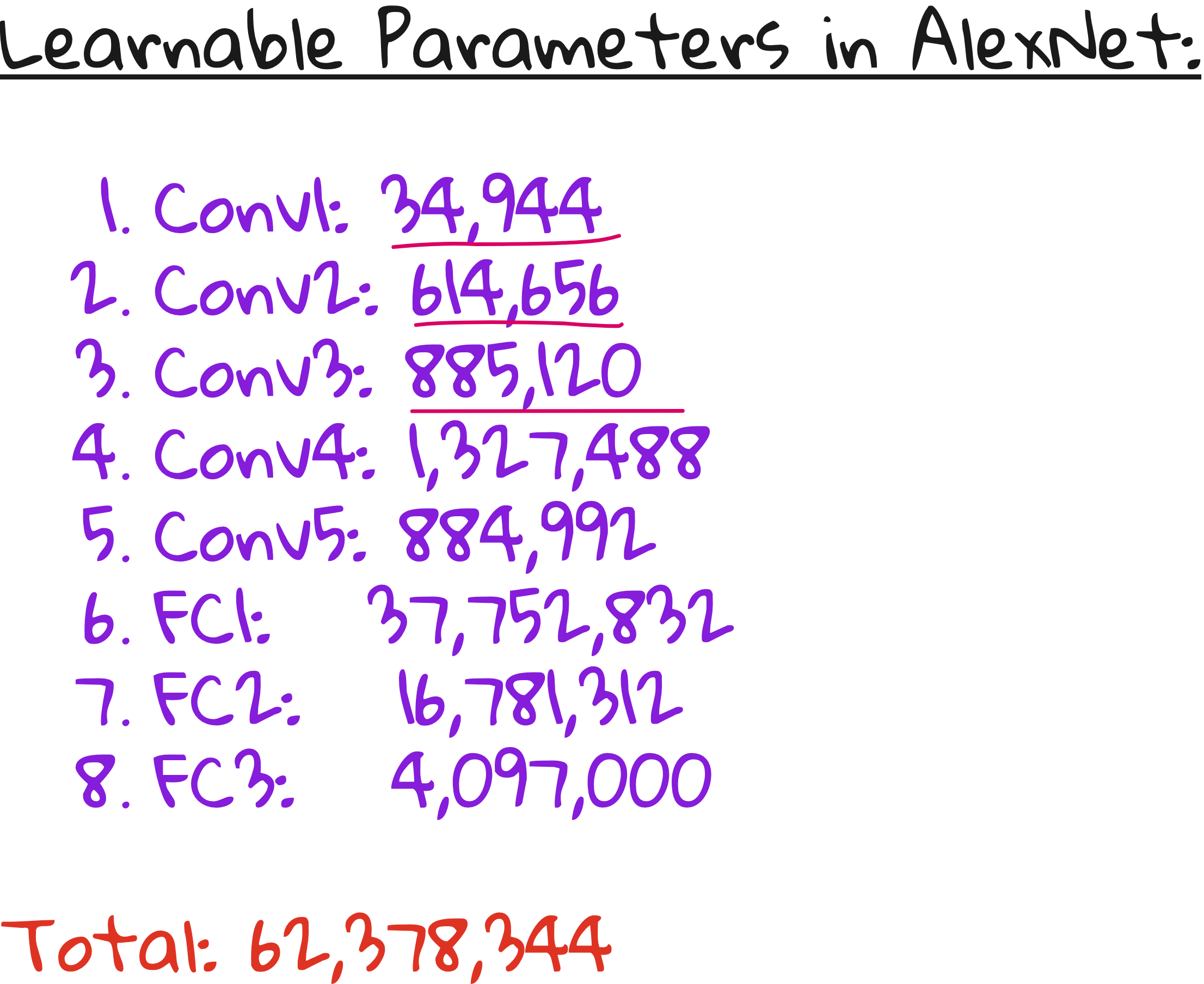
We played with different kernel sizes and strides. Visualized how dimensions change after each operation. Calculated the number of learnable parameters in each layer. (Yes, by hand. With coffee.)

This gave us a strong footing to appreciate what AlexNet does across its 5 convolution layers and 3 fully connected layers.

Implementing AlexNet using pytorch

Finally, we implemented AlexNet using PyTorch.

We used the pretrained version from ImageNet.
Replaced the final layer with a fully connected layer of size 5 (for our flower classes).
Used the Adam optimizer with a learning rate of 0.001.
Ran for 10 epochs with batch size 16.
Logged everything using Weights and Biases.

The results?

Training accuracy: 93–95 percent
Validation accuracy: ~90 percent - the highest we have achieved in the course

Not bad for a model introduced over a decade ago.

So, what did we learn?

AlexNet may not be state-of-the-art today, but it still teaches us foundational lessons:

Deep learning works best when you let the model learn features.
Pretrained models are a superpower.
Understanding convolution at an intuitive level pays off.
And GPUs are not optional.

Most importantly, we learned that good results often come after many failed experiments.

Our journey went from 40 percent to 90 percent validation accuracy - but it passed through regularization, dropout, early stopping, transfer learning, and some serious debugging.