Gradient Descent: An Introduction to Optimization in ML

Optimization in machine learning is like tuning a guitar: you need to know the method and have the intuition. In this article, we’ll explore the principles of optimization, breaking it down into manageable parts, going into mathematical details, and taking a deep dive into advanced techniques for optimization. At the end of this article I also hope to bring some intuition to the way you think about gradient descent for ML.

What Are We Optimizing For?

At its heart, optimization in ML is about minimizing errors. Imagine training a machine learning model as teaching a clumsy apprentice to cook. They keep spilling ingredients, but with every attempt, they (hopefully) improve. Optimization ensures that with enough feedback, they make fewer mistakes over time.

Mathematically, optimization focuses on minimizing (or maximizing) an objective function, which reflects how well your model performs.

In ML, the objective function is often a loss function L(θ) where θ represents the parameters of the model. Our goal? Adjust θ to make L(θ) as small as possible.

What Are ML Model Parameters?

A machine learning model is essentially a mathematical framework for making predictions or decisions. Think of it as a recipe. The parameters (θ) are the ingredients—things you tweak to get the perfect outcome.

For instance:

• In linear regression, parameters are the slope (m) and intercept (c) of the line. Here m and c are collectively called θ.

• In neural networks, parameters include weights (W) and biases (b) connecting different layers. Here W and b are collectively called θ.

These parameters are adjusted during training to improve the model’s accuracy. ML optimization is about finding the best possible model parameters that make predictions very close to real data.

What Is a Loss Function?

The loss function tells the model how far it is from the correct answer. The singular objective of ML is to minimize the loss function.

So what are we minimizing the loss against? The model parameters. The loss function L is a function of model parameters L(θ). So our goal is to find the values of θ that minimizes L(θ).

Depending on the model type, we can define appropriate loss function.

Types of Loss Functions for Different ML Models

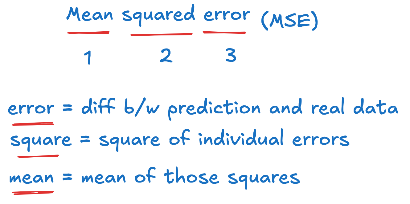
1. Linear Regression:
   Uses Mean Squared Error (MSE):

   \(L(\theta) = \frac{1}{n} \sum_{i=1}^n (y_i - \hat{y}_i)^2 \)

   Mean of square of distance between the true value and the predicted value.

   

2. Logistic Regression & Classification: Employs Cross-Entropy Loss:

   \(L(\theta) = -\frac{1}{n} \sum_{i=1}^n \left[ y_i \log(\hat{y}_i) + (1 - y_i) \log(1 - \hat{y}_i) \right] \)

   This measures the distance between the predicted probability and the true label.

3. Hinge Loss (for SVMs):

\(L(\theta) = \sum_{i=1}^n \max(0, 1 - y_i \hat{y}_i) \)

Hinge loss is used in Support Vector Machines (SVMs) to ensure that predictions are not just correct but confidently so, by penalizing predictions that are close to the decision boundary, encouraging the model to achieve a margin of at least 1 between classes.

Gradient Descent: The Backbone of Optimization

So how do we minimize the loss function L(θ)? Using gradient descent. This is the single most important mathematical concept that underlies every single ML model.

When we plot loss function L(θ) against model parameters θ, it forms a contour. The global minimum of this contour is our ideal solution for θ that optimizes the ML mode. So how do we arrive at this global minimum or one of the acceptable local minima?

Loss function contour plotted as a function of model parameters θ

Imagine standing on a foggy mountainside and trying to reach the valley below by taking small steps downhill. That’s gradient descent in a nutshell.

Mathematical Explanation: Gradient descent updates parameters θ iteratively: θ=θ−η∇L(θ)

Here:

• ∇L(θ): Gradient of the loss function with respect to θ.

• η: Learning rate (how big the steps are).

Steps involved in gradient descent:

Step 1: Start with random value of model parameters

Step 2: Calculate the gradient

Step 3: Update the parameters

Repeat steps 2 and 3 until convergece

Shortcomings of Gradient Descent for Big and Noisy Datasets

Gradient descent isn’t perfect. It can be:

• Slow for large datasets.

• Prone to getting stuck in local minima or saddle points where slope=0.

• Sensitive to noisy data, leading to unstable updates.

• Oscillations when the learning rate (η) is big.

  

Ways to Make Gradient Descent Better

Over time, researchers have refined gradient descent like upgrading from a clunky typewriter to a sleek laptop. The most popular variants include:

Method 1: Stochastic Gradient Descent (SGD)

Method 2: Momentum

Method 3: RMSprop

Method 4: Adam

We will learn these methods in detail in follow-up articles.

Here is a code to implement gradient descent from scratch using a synthetic dataset.

import numpy as np
import matplotlib.pyplot as plt

# Generate a simple dataset (y = 2x + 1 with noise)
np.random.seed(42)
X = np.linspace(0, 10, 50)  # 50 evenly spaced points between 0 and 10
true_m, true_c = 2, 1
y = true_m * X + true_c + np.random.normal(0, 2, X.shape)  # Add some noise

# Initialize parameters (slope and intercept)
m, c = 0.0, 0.0  # Starting with random guesses
learning_rate = 0.01  # Learning rate
iterations = 1000  # Number of iterations

# Store loss for plotting
loss_history = []

# Gradient Descent
for i in range(iterations):
    # Predicted y values
    y_pred = m * X + c
    
    # Compute gradients
    m_grad = (-2 / len(X)) * np.sum(X * (y - y_pred))
    c_grad = (-2 / len(X)) * np.sum(y - y_pred)
    
    # Update parameters
    m = m - learning_rate * m_grad
    c = c - learning_rate * c_grad
    
    # Compute loss (MSE)
    loss = np.mean((y - y_pred) ** 2)
    loss_history.append(loss)
    
    # Print updates every 100 iterations
    if i % 100 == 0:
        print(f"Iteration {i}: Loss = {loss:.4f}, m = {m:.4f}, c = {c:.4f}")

# Print final parameters
print(f"Final parameters: m = {m:.4f}, c = {c:.4f}")

# Plot the dataset and the fitted line
plt.figure(figsize=(10, 6))
plt.scatter(X, y, label="Data Points", color="blue")
plt.plot(X, m * X + c, label=f"Fitted Line: y = {m:.2f}x + {c:.2f}", color="red")
plt.title("Gradient Descent: Line Fitting")
plt.xlabel("X")
plt.ylabel("y")
plt.legend()
plt.show()

# Plot loss history
plt.figure(figsize=(10, 6))
plt.plot(range(iterations), loss_history, label="Loss")
plt.title("Loss Over Iterations")
plt.xlabel("Iterations")
plt.ylabel("Mean Squared Error")
plt.legend()
plt.show()