Equation "discovery" using Machine Learning

Can an ML model truly learn science?

ML has transformed how we make predictions - from recommending songs to detecting diseases. But in many scientific fields, there is a hard truth: data is limited, expensive, or even impossible to collect.

So what do we do when we don’t have big data - but we do have decades of theory?

That is where Scientific Machine Learning (SciML) comes in. It blends physics with neural networks, math with models, equations with gradients. And at the heart of this field is a concept that is elegant, flexible, and wildly powerful:

Universal Differential Equations (UDEs).

What is the problem with traditional ML scene?

Let us start with a familiar picture. In domains like bioinformatics or social networks, you can build powerful models because you have terabytes of data. But try doing that in:

• Astronomy (telescope time is expensive)

• Quantum mechanics (experiments are rare and noisy)

• Climate science (you only have one Earth)

And things start to fall apart. Worse still:

• You might have equations that partially describe your system…

• But they ire too simplistic. Too many assumptions. Or too rigid for the real world.

So where do we go from here?

The philosophy behind Scientific ML

“A model is worth a thousand datasets.”

If you have a governing equation - even an incomplete one - you already have something extremely valuable: structure. That structure encodes causality, symmetry, and physical intuition that no amount of pure data-driven ML can learn.

What Scientific Machine Learning does is simple, yet profound:

• It keeps what you know (mechanistic models)

• It learns what you don’t (via neural nets)

• And it does this in a way that is interpretable, efficient, and scalable

Enter Universal Differential Equations (UDEs)

At a high level, a UDE is just a differential equation where part of the right-hand side is replaced by a neural network.

UDEs are differential equations which are defined in full or part by a universal approximator.

A universal approximator is a parameterized object capable of representing any function.

Let us break it down with an example.

Classic Heat Equation (1D)

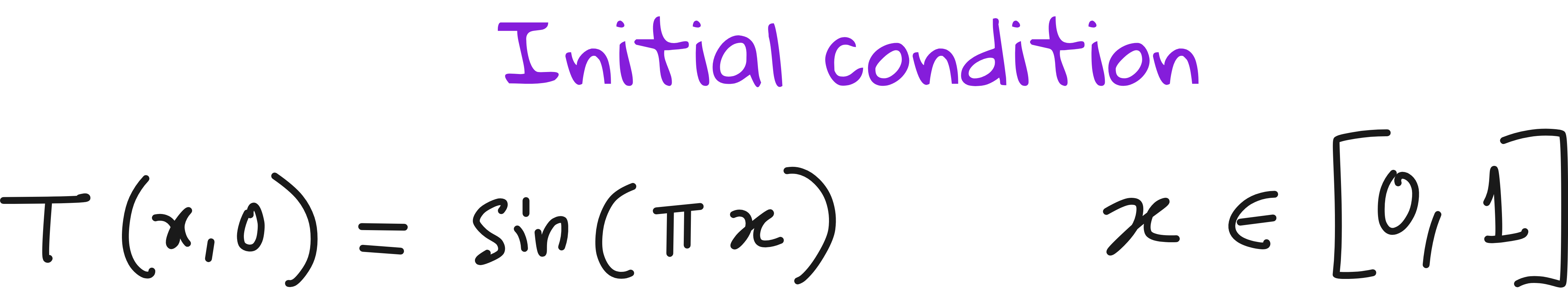
Say we have a rod of length L, and we want to model how temperature T(x,t) evolves over time.

In classical PDEs, you must know the exact form of all physical terms (e.g. diffusion constant D, spatial discretization - 2nd order derivative).

Where:

• T(x,t): temperature at location x and time t

• D: diffusion coefficient (assumed constant)

Assuming periodic or circular boundary conditions, this rod redistributes heat over time such that hotter regions cool down and cooler regions heat up.

UDE Version

But what if we don’t know D?
What if the material is heterogeneous? Or there is some hidden heat source?

We turn this into a learning problem by embedding learnable components into the PDE:

1. Allow the model to learn the diffusion term and stencil directly from data.

2. Retain the physical structure of a heat equation (i.e. time evolution from spatial gradients).

2 learnable components

1. Learnable Diffusion Coefficient (D)

Instead of assuming a fixed value for ddd, we model it as a scalar neural network parameter - learned from data. It is like saying:

“I believe diffusion is happening, but I’ll let the data tell me how much.”

This is a perfect example of physics-informed learning.

2. Learnable Spatial Operator (Using a CNN)

Now here’s where things get spicy:
To compute the second spatial derivative​, we don’t use finite differences directly.

Instead, we use a convolutional neural network (CNN).

Why? Because convolution is just a generalized form of a numerical stencil.

A stencil is a set of weights applied to neighboring points to estimate derivatives.

Example: To approximate ∇^2(T)​, the classic 3-point stencil is: [1,-2,1]

What is a stencil, really?

Here is a simple analogy:

• In image processing, a convolution kernel (like [−1, 0, 1]) detects edges.

• In scientific computing, a stencil (like [1, -2, 1]) detects curvature.

Both are local operators applied over a window of data.

In our UDE, we use a learnable stencil (i.e., a 1D CNN kernel) to approximate the spatial behavior of T(x). This could be:

• Second derivative (diffusion)

• First derivative (advection)

• Something more complex (if physics is nonlocal)

By letting the stencil weights be trainable, the network can learn whether the underlying dynamics are closer to Laplacian, biharmonic, or something entirely new.

We can derive the stencil for the second derivative as following.

You may have 2 questions

Why are we recovering only 2 terms?

What is the format of this learnable stencil in 1D heat equation?

Let us discuss these 2 questions.

Why only 2 terms?

Why, in this UDE setup for the 1D heat equation, are we only learning the diffusion coefficient D and the stencil weights? Why not other terms?

1. You assume no local reaction term. The system is governed only by diffusion. There is no advection, or forcing term.

2. You assume the process is pure diffusion that depends on some kind of spatial temperature distribution and some diffusion coefficient.

Structuring the UDE neural network

So why use a 3-point stencil?

Even without assuming it’s the Laplacian, you choose a 3-point stencil for three reasons:

1. Locality assumption: You are assuming that the operator depends on a small neighborhood (e.g., 3 adjacent points).

2. Model simplicity: 3-point stencil is the simple nontrivial operator

3. Exploratory goal: You test if the data explained by a 2nd-derivative-like operator?

So in UDE, you start simple, let the data guide you, and expand later if necessary.

We should also enforce the sum of stencil weights = 0

In physical systems governed by diffusion (e.g., heat or particles), mass or energy must be conserved in the absence of sources or sinks.

Because this is over the whole domain (with periodic or zero-flux boundary conditions), shifting the indices doesn’t change the total sum. So:

Thus we can rewrite the equation as:

Loss function

Our loss function has 3 parts.

1. Mean squared error due to the difference in predicted and actual temperature

2. Loss due to diffusion term

3. Loss to enforce sum of weights to be zero.

So how do we calculate each of these?

1. Prediction Loss (Mean Squared Error - MSE)

What it measures:

This part of the loss evaluates how well the model's predicted temperature field matches the actual temperature field (ground truth) over time.

2. Diffusion Term Loss

What it measures:

This penalizes the deviation of the learned diffusion coefficient D from a known or expected value​. Useful when you have some prior knowledge about how fast diffusion should happen.

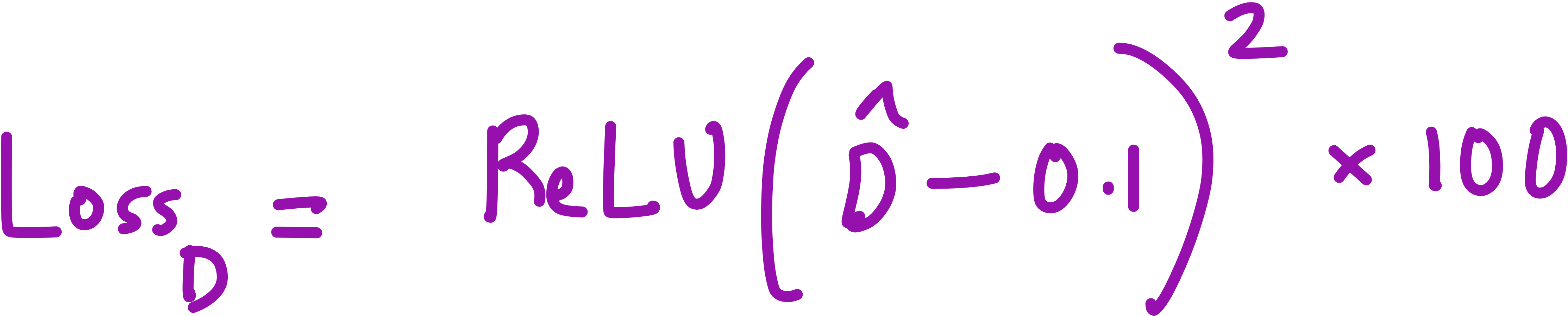
3. Stencil Conservation Loss (Sum of Weights = 0)

What it measures:

This term ensures that the stencil (i.e., the weights of the convolutional kernel) respects conservation laws like mass conservation, by having their sum be zero.

Total loss: Sum of all 3 losses

What does the neural network look like?

Input

The input to your CNN is a sliding window over the spatial grid of your PDE solution, T(x, t). Since the convolutional layer uses a 3-tap kernel ((3, 1, 1, 1)), at each spatial location xₖ, it takes: [Tₖ₋₁, Tₖ, Tₖ₊₁].

This is essentially a 3-point stencil used to approximate a spatial derivative (like the Laplacian).

We can draw the structure of the neural network as shown below. The initial input is the temperature initial conditions.

This input is acted upon by the stencil to produce a single number that represents the Laplacian.

This number is scaled by the learned D to get the approximate value of rate of change of temperature.

This can be numerically integrated to get predicted values of temperature.

In our modeling we use:-

• Initial weights: [1.1, -2.5, 1.0] - this resembles a second derivative stencil.

• Initial bias: [0.0] - no bias added.

• Padding: None, meaning output is reduced near the boundaries.

Results

I run the Universal PDE to get the results shown below. The full code is give in the appendix.

Original UDE paper from MIT

https://arxiv.org/pdf/2001.04385

Interested in publishing SciML research paper? Check this out

https://flyvidesh.online/ml-bootcamp/

Lecture video

I have made a lecture video on this topic and hosted it on Vizuara’s YouTube channel. Do check this out. I hope you enjoy watching this lecture as much as I enjoyed making it.

Full code

Import packages

###############################################################################
# USING PACKAGES
###############################################################################

using PyPlot
using Printf
using LinearAlgebra
using Flux, DiffEqFlux, Optim, SciMLSensitivity
using OrdinaryDiffEq
using ComponentArrays
using Random
using BSON: @save, @load
using Optimization, OptimizationOptimJL, OptimizationOptimisers

Problem setup

###############################################################################
# PROBLEM SETUP
###############################################################################

# PDE parameters
D = 0.1            # True diffusion coefficient
X = 1.0             # 1D domain length
T = 0.5             # Simulation time
dx = 0.01
dt = T/10
x = collect(0:dx:X)
t = collect(0:dt:T)
Nx = Int64(X/dx+1)
Nt = Int64(T/dt+1)

# Initial condition: Sinusoidal
rho0 = @. sin(π*x)

save_folder = "data"

if isdir(save_folder)
    rm(save_folder, recursive=true)
end
mkdir(save_folder)

Simulated ground truth

###############################################################################
# GENERATE TRAINING DATA FROM TRUE HEAT PDE
###############################################################################

lap = diagm(0 => -2.0*ones(Nx),
            1 =>  ones(Nx-1),
           -1 =>  ones(Nx-1)) / dx^2
lap[1,end] = 1.0/dx^2
lap[end,1] = 1.0/dx^2

function heat_rhs(rho, p, t)
    D * (lap * rho)
end

prob_data = ODEProblem(heat_rhs, rho0, (0.0, T), saveat=dt)
sol_data  = solve(prob_data, Tsit5())
ode_data  = Array(sol_data)

fig = figure(figsize=(8,3))
sub1 = fig.add_subplot(1,2,1)
pcolormesh(x, t, ode_data')
sub1.set_xlabel("x")
sub1.set_ylabel("t")
fig.colorbar(PyPlot.gci(), ax=sub1)
sub1.set_title("Heat Equation Data")

sub2 = fig.add_subplot(1,2,2)
for i in 1:2:Nt
    sub2.plot(x, ode_data[:, i], label="t=$(sol_data.t[i])")
end
sub2.set_xlabel("x")
sub2.set_ylabel(L"\rho")
sub2.legend(fontsize=7, loc="upper left", bbox_to_anchor=(1,1))
sub2.set_title("Slices of solution")
tight_layout()
fig.savefig(joinpath(save_folder, "training_data.pdf"))

Animated temperature evolution

###############################################################################
# ANIMATE HEAT DIFFUSION AS GIF
###############################################################################

using Plots
gr()  # use GR backend
anim = @animate for i in 1:Nt
    Plots.plot(x, ode_data[:, i],
         ylim=(0, maximum(ode_data)),
         xlabel="x", ylabel="Temperature ρ(x,t)",
         title = @sprintf("Heat Diffusion at t = %.2f", t[i]),
         linewidth=3, legend=false)
end

gif_path = joinpath(save_folder, "heat_diffusion.gif")
gif(anim, gif_path, fps=10)

Define the Neural network + PDE

###############################################################################
# DEFINE THE NEURAL PDE (ONLY DIFFUSION)
###############################################################################
p
init_w = reshape([1.1, -2.5, 1.0], (3,1,1,1))
diff_cnn_flux = Flux.Conv(init_w, [0.0], pad=(0,0,0,0))
p1, re1 = Flux.destructure(diff_cnn_flux)

D0_init = [0.0]
p_init = [p1; D0_init]

function full_restructure(pvec)
    cnn_len = length(p1)
    diff_cnn_ = re1(pvec[1:cnn_len])
    D0_ = pvec[end]
    return diff_cnn_, D0_
end

Neural PDE, prediction and loss

###############################################################################
# NEURAL PDE ODE FUNCTION
###############################################################################

function nn_ode!(drho, rho, p, t)
    diff_cnn_, D0_ = full_restructure(p)
    w1, w2, w3 = diff_cnn_.weight[:]

    @inbounds for i in 1:Nx
        left  = (i == 1)  ? Nx : (i - 1)
        right = (i == Nx) ? 1  : (i + 1)
        drho[i] =  D0_ * (w1*rho[left] + w2*rho[i] + w3*rho[right]) / (dx^2)
    end
end

###############################################################################
# PREDICTION & LOSS
###############################################################################

prob_nn = ODEProblem(nn_ode!, rho0, (0.0, T), p_init)

function predict_nn(p)
    sol = solve(prob_nn, Tsit5();
                p=p, dtmax=dt, saveat=t,
                sensealg=InterpolatingAdjoint(autojacvec=ReverseDiffVJP()),
                abstol=1e-9, reltol=1e-9, maxiters=1e6)
    Array(sol)
end

function loss_nn(p)
    pred = predict_nn(p)
    diff_cnn_, D0_ = full_restructure(p)
    w = diff_cnn_.weight[:]
    
    D0_penalty = 500 * relu(D0_ - 0.1)^2
    kernel_penalty = 100 * abs(sum(w))
    # return sum(abs2, ode_data .- pred) + kernel_penalty 
    return sum(abs2, ode_data .- pred) + kernel_penalty + D0_penalty
end

function loss_nn_adam(p, args...)
    loss_nn(p)
end

###############################################################################
# CALLBACK
###############################################################################

global train_losses = Float64[]
global epoch_count = 0

function mycallback(state, l; doplot=true)
    global epoch_count
    push!(train_losses, l)
    pcurrent = state.u
    diff_cnn_, D0_ = full_restructure(pcurrent)
    w = diff_cnn_.weight[:]
    @info "Epoch = $epoch_count | Loss = $l | D0 = $D0_ | w= $w | sum(w)= $(sum(w))"
    epoch_count += 1
    return false
end

Optimization

###############################################################################
# OPTIMIZATION
###############################################################################

rng = Xoshiro(42)
p0 = copy(p_init)

@info "Starting ADAM training on Heat Equation..."

adtype = Optimization.AutoZygote()
optf_adam = Optimization.OptimizationFunction(loss_nn_adam, adtype)
optprob_adam = Optimization.OptimizationProblem(optf_adam, p0)

res_adam = Optimization.solve(
    optprob_adam,
    OptimizationOptimisers.Adam(0.01);
    maxiters=200,
    callback = (state, L)->mycallback(state, L; doplot=false)
)

Final plots

###############################################################################
# SAVE & FINAL PLOTS
###############################################################################

pstar = res_adam.u

@save joinpath(save_folder, "heat_model.bson") pstar
# pstar = [1.0, -2.0, 1.0, 0.0, 0.01]

pred_data2 = predict_nn(pstar)

# Compare data vs prediction
figf = figure(figsize=(8,3))
subA = figf.add_subplot(1,2,1)
pcolormesh(x, t, ode_data')
subA.set_xlabel("x")
subA.set_ylabel("t")
figf.colorbar(PyPlot.gci(), ax=subA)
subA.set_title("Reference Data")

subB = figf.add_subplot(1,2,2)
pcolormesh(x, t, pred_data2')
subB.set_xlabel("x")
subB.set_ylabel("t")
figf.colorbar(PyPlot.gci(), ax=subB)
subB.set_title("NN PDE Prediction")
tight_layout()
figf.savefig(joinpath(save_folder, "heat_prediction.pdf"))

# Line slices
fig2 = figure()
PyPlot.plot(x, ode_data[:,1], label="Data t=0")
PyPlot.plot(x, pred_data2[:,1], "--", label="NN t=0")

for i in 2:2:Nt
    PyPlot.plot(x, ode_data[:,i], label="Data t=$(round(t[i],digits=1))")
    PyPlot.plot(x, pred_data2[:,i], "--", label="NN t=$(round(t[i],digits=1))")
end

PyPlot.xlabel("x")
PyPlot.ylabel(L"\rho")
PyPlot.legend()
PyPlot.title("Line slices comparison")
fig2.savefig(joinpath(save_folder, "heat_line_slices.pdf"))

# CNN weights
diff_cnn_, D0_ = full_restructure(pstar)
wfinal = diff_cnn_.weight[:]
@info "Final CNN weights = $wfinal, sum(w)=$(sum(wfinal)), D0 = $D0_"

# Training loss history
fig4 = figure()
PyPlot.plot(0:length(train_losses)-1, log10.(train_losses), "k.-", label="log10(loss)")
PyPlot.xlabel("Epoch")
PyPlot.ylabel("log10(loss)")
PyPlot.title("Training Loss")
PyPlot.legend()
fig4.savefig(joinpath(save_folder, "heat_loss_history.pdf"))

Animated GIF comparing ground truth and NN prediction

using Plots
gr()

anim = @animate for i in 1:Nt
    Plots.plot(x, ode_data[:, i], label="Ground Truth", lw=3, color=:black,
         xlabel="x", ylabel=L"\rho(x, t)",
         title=@sprintf("Heat Diffusion at t = %.2f", t[i]),
         ylims=(0, 1.1 * maximum(ode_data)), legend=:topright)

    Plots.plot!(x, pred_data2[:, i], label="NN Prediction", lw=3, linestyle=:dash, color=:red)
end

gif_path = joinpath(save_folder, "heat_diffusion_comparison.gif")
gif(anim, gif_path, fps=5)