Detection Transformer (DETR): An introduction

How to use transformer for object detection from images?

Jan 15, 2026

Table Of Content

Introduction to DETR
What Is Object Detection
Core Components of an Object Detection Prediction
Object Detection Versus Classification
Anchor Boxes and Non Maximum Suppression
The Detection Transformer (DETR): Architecture and Design Philosophy
Hungarian Matching Loss in Detection Transformers
When Hungarian Matching Is Needed and When It Is Not in DETR
The Limitation of IoU and the Motivation for Generalized IoU
The DETR Loss Function: Formal Definition and Training Mechanics
Concluding Perspective on DETR

1.1 Introduction to DETR

Object detection has historically evolved through increasingly sophisticated architectures that balance localization accuracy, classification performance, and computational efficiency. Detection Transformers represent a conceptual shift in this progression. Instead of relying on handcrafted components such as anchor boxes, region proposal pipelines, or dense sliding window predictions, detection transformers formulate object detection as a direct set prediction problem. By leveraging the transformer architecture, these models jointly reason about global image context and object relationships, enabling a simpler and more unified detection pipeline. While the core ideas are not mathematically complex, detection transformers require careful attention to how multiple components interact, including feature extraction, set based prediction, and loss formulation. This section builds the foundation needed to understand detection transformers by first revisiting object detection itself from first principles.

1.2 What Is Object Detection

Figure 1.1 Example of object detection output showing multiple bounding boxes, class labels, and confidence scores predicted within a single image.

Object detection extends image classification by moving from a single global prediction to multiple localized predictions within the same image. Rather than assigning one label to an entire image, an object detection model identifies and localizes multiple objects, each potentially belonging to a different class. This means that, within one image, the model must reason about several objects simultaneously, their spatial locations, and their semantic categories.

Figure 1.1 illustrates a typical object detection output. Multiple bounding boxes are drawn over the image, each corresponding to a detected object such as a person, a horse, or a dog. Along with each bounding box, the model produces a class label and a confidence score that reflects how strongly the model believes the object belongs to that class.

This differs fundamentally from standard image classification, where the entire image is treated as a single entity. In classification, the output is usually a probability distribution over classes for the whole image. In detection, predictions are localized and repeated across different regions of the image.

1.3 Core Components of an Object Detection Prediction

In object detection, each detected object is described by a compact numerical representation that jointly encodes its spatial location and semantic identity. Unlike image classification, where a single prediction summarizes the entire image, object detection produces multiple localized predictions, one for each object instance. Each prediction must therefore be expressive enough to specify where the object is and what it represents, while remaining simple enough to be learned efficiently.

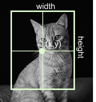
Figure 1.2 Bounding box parameterization for object detection, showing the object represented by the center coordinates (x,y) along with its width and height, which together uniquely define the spatial extent of the detected object within the image.

The spatial extent of an object is captured through a bounding box. A bounding box is uniquely defined by four continuous parameters: the x and y coordinates of its center, along with its width and height. This representation is minimal and sufficient to reconstruct the rectangular region corresponding to the object. In practice, these values are normalized with respect to the image dimensions so that they lie in the range from zero to one, which simplifies optimization and allows the model to generalize across images of different resolutions.

Beyond localization, the model must also assign a semantic label to the contents of each bounding box. This is achieved by predicting a probability distribution over the predefined set of object classes. The distribution reflects the model’s relative confidence across all possible categories and forms the basis for deciding which class is ultimately assigned to the detected object.

Finally, object detection models associate each prediction with a confidence score that reflects the likelihood that a valid object is present at the predicted location. This score plays a crucial role during inference, where low confidence predictions are typically discarded to reduce false positives. Depending on the model design, this confidence may be predicted explicitly or implicitly encoded within the class probabilities.

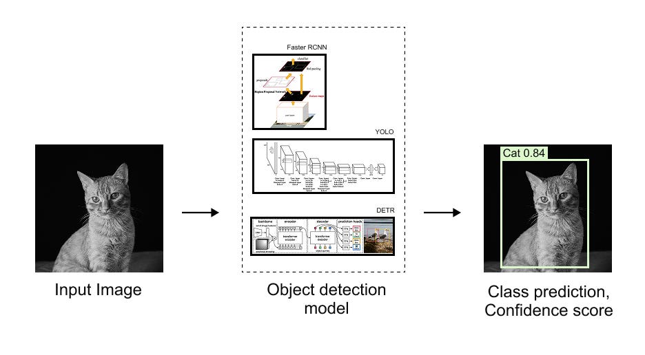
Figure 1.3 High level object detection pipeline illustrating how an input image is processed by an object detection model to produce localized bounding boxes, along with corresponding class predictions and confidence scores.

1.4 Object Detection Versus Classification

The distinction between object detection and image classification becomes clear when examining the structure of their model outputs and the losses used during training. In a standard classification task, the model processes an entire image as a single unit and produces a probability vector over the available classes. The corresponding ground truth is typically represented as a one hot encoded vector, and learning is driven by a cross entropy loss that measures the discrepancy between the predicted probability distribution and the true class label.

Object detection introduces additional complexity because the model must solve multiple prediction problems simultaneously. In addition to assigning a class label, the model must also predict continuous values that describe the spatial extent of each object, such as the bounding box coordinates. As a result, detection models rely on composite loss functions that integrate several objectives into a single training signal. These typically include a classification loss that supervises the predicted class probabilities, a regression loss that penalizes errors in the predicted bounding box parameters, and, in many formulations, an additional objectness or confidence loss that reflects whether a predicted region corresponds to a real object.

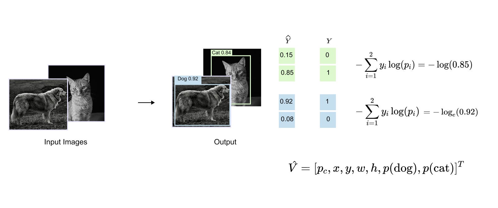
Figure 1.4 illustrates this idea in the context of class prediction, showing how the model outputs a probability distribution for each detected object and how this distribution is compared against the one hot encoded ground truth using a cross entropy loss. Together, these loss components enable object detection models to jointly learn accurate localization and reliable classification within a unified optimization framework.

From a purely conceptual standpoint, an object detection model can be seen as a function that maps an image to a set of vectors, where each vector encodes one detected object. In the simplest case, one might imagine a neural network that takes an image and outputs a single detection vector. This approach quickly breaks down in realistic settings, as images often contain multiple objects, possibly of the same class, and in varying spatial configurations.

This limitation motivated earlier detection architectures such as Faster R CNN and YOLO, which introduced mechanisms for handling multiple objects through region proposals or dense predictions. These approaches rely heavily on convolutional inductive biases and task specific design choices.

Detection transformers take a different route. They remove many of these handcrafted components and instead rely on the transformer’s ability to model sets and global relationships. Before diving into that architecture, it is essential to be comfortable with the fundamental structure of object detection outputs, targets, and losses, as developed in this section.

1.5 Anchor Boxes and Non Maximum Suppression

Before the introduction of detection transformers, most object detection systems relied on a set of carefully engineered components to handle the challenges of localization and duplicate predictions. Two of the most important of these components were anchor boxes and non maximum suppression. While effective in practice, both mechanisms introduced additional complexity and a significant amount of human design choices into the detection pipeline. Understanding them provides useful historical context and clarifies what detection transformers deliberately remove.

Anchor boxes were introduced as a way to simplify the problem of predicting bounding boxes. Instead of asking a model to predict bounding box coordinates from scratch, earlier detectors predefined a large collection of reference boxes at fixed locations in the image. These reference boxes, called anchor boxes, were placed on a regular grid over the image and instantiated with multiple sizes and aspect ratios at each grid point. The intuition was that, for any object in the image, at least one anchor box would roughly overlap with it. During training, the model learned to slightly adjust the position and shape of these anchor boxes so that they aligned more closely with the ground truth objects.

Figure 1.4 illustrates this idea. At a single spatial location, multiple anchor boxes with different aspect ratios are defined. Some boxes are nearly square, while others are elongated horizontally or vertically. By starting from these diverse shapes, the model can better handle objects with varying geometries, including extreme aspect ratios that arise due to viewpoint changes or object pose.

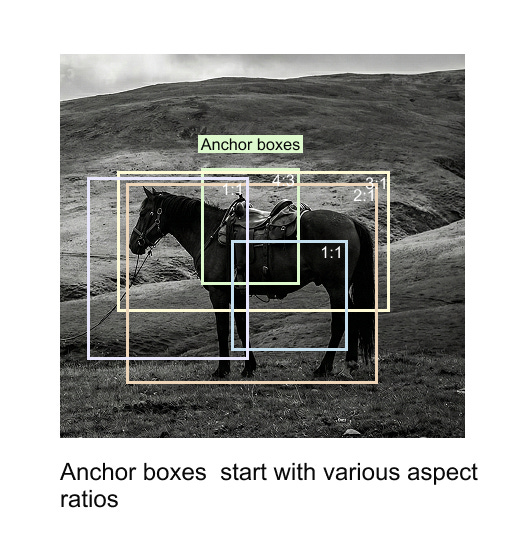
Figure 1.5 Anchor boxes defined at a fixed location with multiple sizes and aspect ratios, serving as predefined starting points for bounding box regression.

While anchor boxes help with localization, they also introduce a side effect. During inference, many anchor boxes may produce very similar predictions for the same object. As a result, a detector often outputs multiple overlapping bounding boxes that all correspond to a single object. This redundancy must be resolved before producing the final set of detections. Non maximum suppression, commonly abbreviated as NMS, was designed to address this problem.

Non maximum suppression is a post processing algorithm applied after the model has produced its raw bounding box predictions. The algorithm operates on a set of predicted boxes, each associated with a confidence score. The first step is to discard boxes whose confidence falls below a predefined threshold. This threshold is chosen manually and reflects the minimum confidence required for a prediction to be considered meaningful. After this filtering step, the remaining boxes are sorted in descending order of confidence.

Figure 1.5 shows the effect of this process. Before non maximum suppression, many overlapping boxes are present around the same object. After applying NMS, only a single bounding box remains, corresponding to the highest confidence prediction.

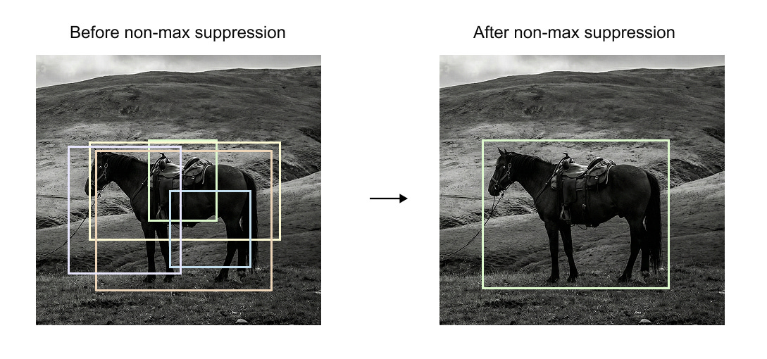
Figure 1.5 Effect of non maximum suppression. Multiple overlapping predictions before NMS are reduced to a single high confidence bounding box after NMS.

The core operation in non maximum suppression is the comparison of bounding boxes using the intersection over union metric, commonly abbreviated as IoU. Given two bounding boxes B_i and B_j, the IoU is defined as the ratio of the area of their intersection to the area of their union,

\( \text{IoU}(B_i, B_j) = \frac{\text{Area}(B_i \cap B_j)}{\text{Area}(B_i \cup B_j)} \)

This value lies between zero and one. An IoU of zero indicates no overlap, while an IoU of one indicates perfect overlap. Figure 1.6 provides a visual interpretation of IoU, along with examples of high, moderate, and low overlap scenarios.

Figure 1.6
Intersection over Union illustrated as the ratio between overlapping area and total union area, with examples ranging from excellent to poor overlap.

Using IoU, non maximum suppression proceeds iteratively. The box with the highest confidence score is selected and added to the final output set. This box is then compared with all remaining boxes. Any box whose IoU with the selected box exceeds a predefined IoU threshold is removed, as it is considered a duplicate prediction of the same object. Boxes with low IoU values, such as 0.1 or 0.2, are retained because they likely correspond to different objects. The process is then repeated with the next highest confidence box among the remaining predictions, continuing until no boxes remain.

Figure 1.7 summarizes this algorithmic flow, highlighting how confidence thresholds and IoU thresholds guide the suppression process.

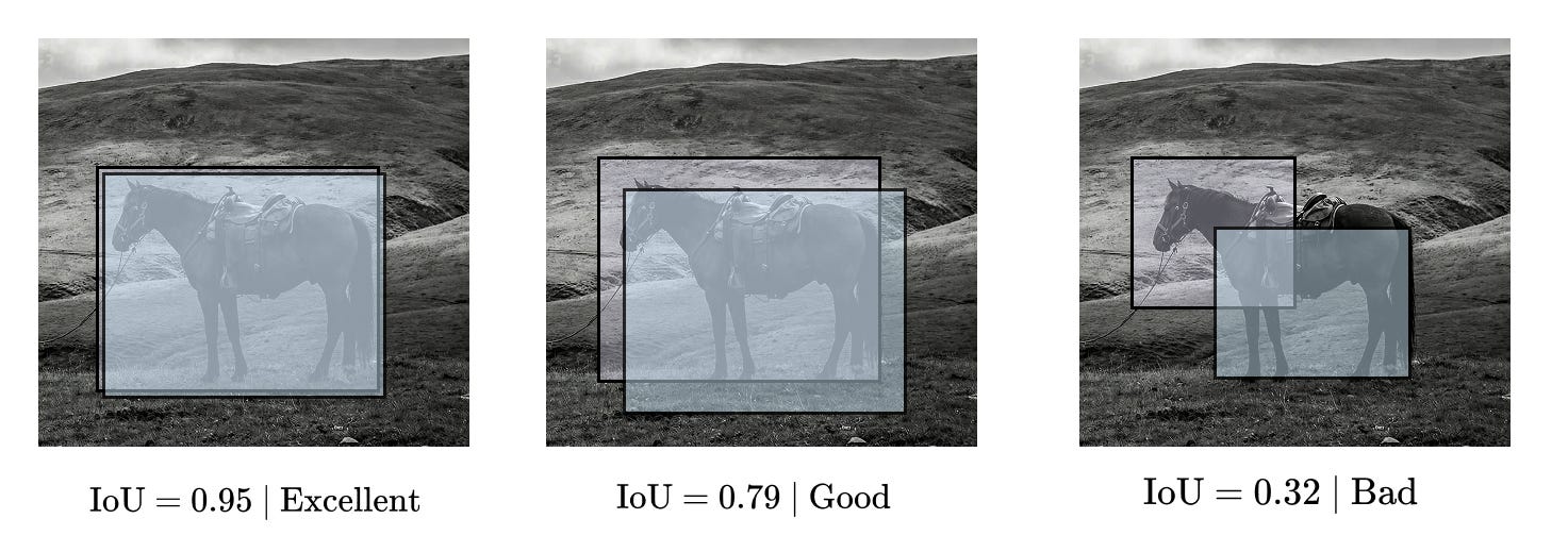
Figure 1.7
Step by step procedure of non maximum suppression, including confidence filtering, IoU computation, and iterative removal of duplicate boxes.

Although effective, both anchor boxes and non maximum suppression rely heavily on hand engineered choices. The number of anchor boxes, their aspect ratios, the confidence threshold, and the IoU threshold are all selected manually, typically through trial and error. These design decisions are not learned from data and can significantly influence detection performance. Detection transformers remove both anchor boxes and non maximum suppression, replacing them with a learned set based prediction mechanism. This shift toward end to end learning is one of the central motivations behind the detection transformer architecture and will be explored in detail in the following sections.

1.6 The Detection Transformer (DETR): Architecture and Design Philosophy

The Detection Transformer (DETR) represents a conceptual shift in object detection by reformulating detection as a direct set prediction problem. Unlike traditional detectors that rely on dense proposals, anchor boxes, and post-processing steps such as non-maximum suppression, DETR predicts a fixed-size set of object candidates in a single forward pass and matches them globally to ground-truth objects using a set-based loss. This design eliminates hand-engineered components and allows object detection to be expressed entirely within an end-to-end trainable framework built around the transformer encoder–decoder architecture.

At a high level, DETR consists of four major components: a convolutional backbone for feature extraction, a transformer encoder for global contextual reasoning, a transformer decoder driven by object queries, and lightweight prediction heads that output class labels and bounding boxes. The interaction between these components enables DETR to jointly reason about object presence, category, and spatial localization.

Figure 1.8 Overall architecture of the Detection Transformer (DETR), illustrating the flow from input image to CNN feature extraction, transformer encoder–decoder processing, and final set-based object predictions.

From Image to Feature Map: CNN Backbone Representation

The DETR pipeline begins with an input image, which is first processed by a standard convolutional neural network such as ResNet-50 or ResNet-101. This backbone is typically pretrained on ImageNet and serves the purpose of extracting rich, hierarchical visual features from the image. As the image propagates through successive convolutional layers, its spatial resolution is progressively reduced while the number of feature channels increases.

The resulting output is a feature map of shape

\((H_f \times W_f \times C)\)

where H_f and W_f are the reduced spatial dimensions and C is the number of channels.

These feature maps encode semantic and spatial information about the image, but they are still arranged in a two-dimensional grid. Since transformers operate on sequences rather than grids, this representation must be transformed before it can be processed by the encoder.

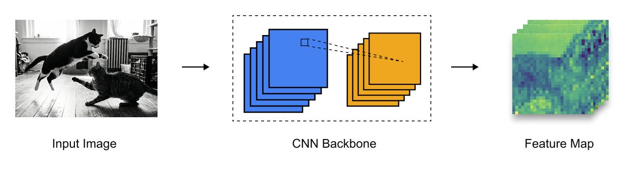
Figure 1.9 Conversion of an input image into a dense feature map using a CNN backbone, where spatial resolution is reduced and semantic richness is increased.

Tokenization and Positional Encoding of Image Features

To make the CNN feature map compatible with the transformer encoder, the spatial grid of features is flattened into a one-dimensional sequence. Each spatial location in the feature map is treated as a token, resulting in a sequence of length

\(H_f \times W_f\)

Before feeding this sequence into the transformer, a linear projection is applied to map each feature vector from channel dimension C into the transformer’s embedding dimension d_model

Because transformers lack an inherent notion of spatial order, positional information must be explicitly injected. DETR employs sinusoidal positional encodings, derived from the original Transformer formulation, to encode the two-dimensional spatial position of each feature token. These positional encodings are added to the token embeddings and are injected at every transformer encoder layer, ensuring that spatial information is preserved throughout the encoding process.

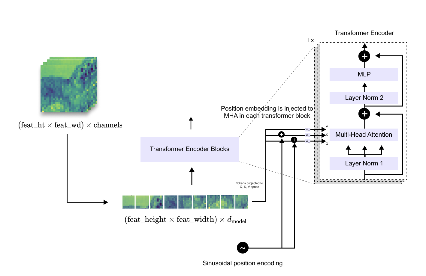
Figure 1.10 Flattening of CNN feature maps into a sequence of tokens and the addition of sinusoidal positional encodings prior to transformer encoding.

While the encoder processes image-derived tokens, the transformer decoder in DETR introduces a fundamentally different concept: object queries. Object queries are a fixed set of learnable vectors, initialized independently of the input image, whose number determines the maximum number of objects the model can predict. For example, if 100 object queries are used, the model will always produce 100 predictions, regardless of how many objects are actually present in the image.

These object queries act as slots that compete to explain objects in the scene. Some queries will eventually specialize to predict real objects, while others will learn to predict the special “no-object” class, corresponding to background.

The decoder processes object queries through multiple decoder blocks, each consisting of three main sublayers: self-attention among object queries, cross-attention between object queries and encoder outputs, and a feed-forward network. In the self-attention stage, object queries interact with each other, allowing the model to reason about relationships between predicted objects and to avoid redundant detections. In the cross-attention stage, object queries attend to the encoder’s image representations, enabling each query to focus on relevant regions of the image.

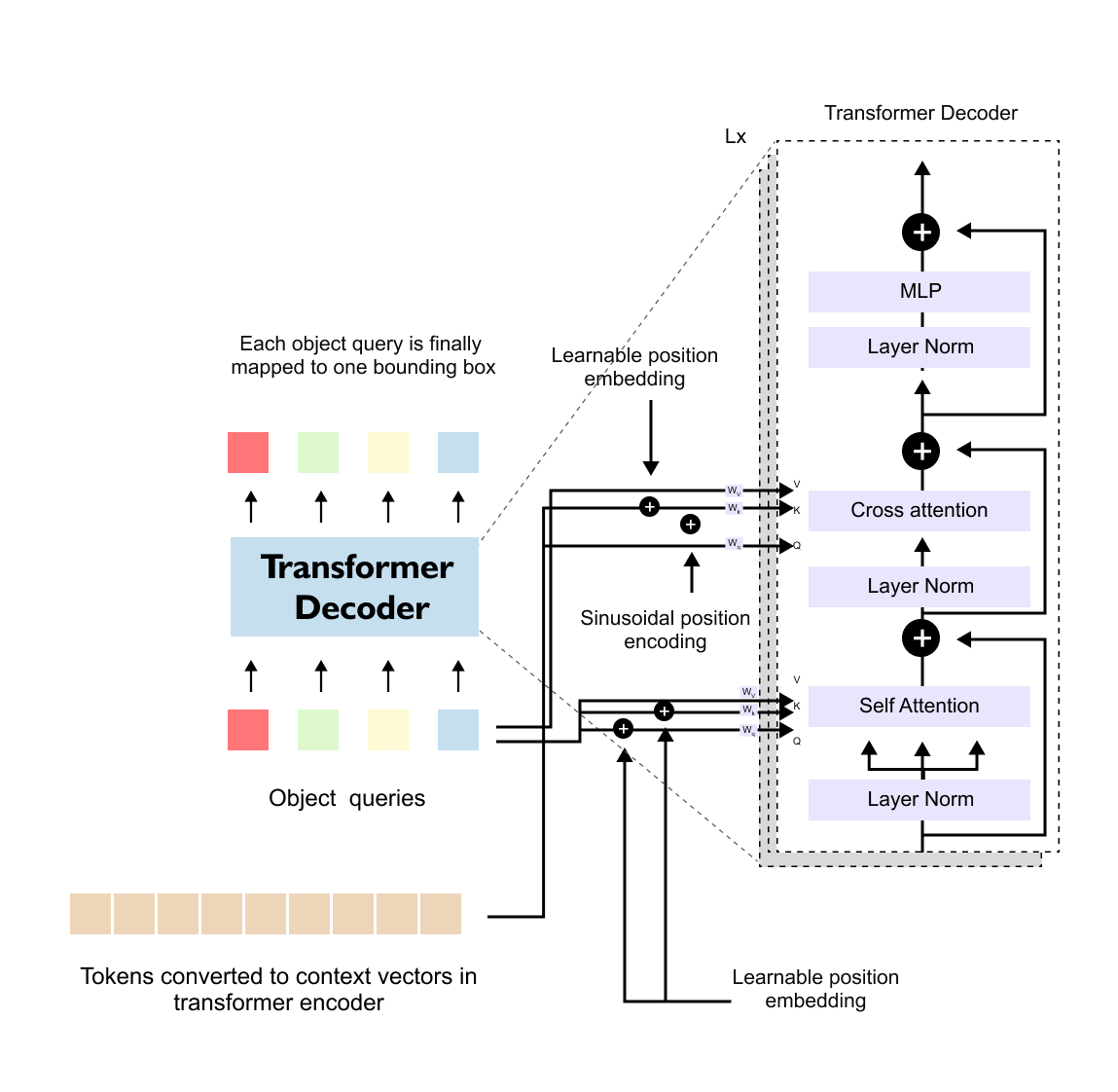
Figure 1.11 Transformer decoder structure in DETR, illustrating self-attention among object queries and cross-attention in DETR, highlighting the different origins of queries (object queries) and keys/values (encoder outputs).

Cross-Attention and Query–Key–Value Asymmetry

A key distinction between the transformer encoder and decoder lies in the source of queries, keys, and values. In encoder self-attention, all three originate from the same sequence of image tokens. In contrast, during decoder cross-attention, the queries originate from object queries, while the keys and values originate from the encoder’s output representations of the image. This asymmetry is what defines cross-attention and allows object queries to selectively extract information from the image.

Unlike image tokens, object queries do not have an inherent spatial ordering. As a result, DETR uses learnable positional embeddings for object queries instead of sinusoidal ones. These embeddings are trained jointly with the rest of the model and allow the decoder to differentiate between individual query slots.

Prediction Heads and Set-Based Outputs

After passing through the transformer decoder, each object query is transformed into a final embedding that is fed into two lightweight feed-forward networks. One prediction head outputs a probability distribution over object classes, including a special background class, while the other predicts the bounding box parameters (x, y, w, h) in normalized image coordinates.

Crucially, there is a one-to-one correspondence between object queries and predictions: each query produces exactly one class prediction and one bounding box. The full output of DETR is therefore a set of predictions, whose size is fixed by design and independent of the image content.

Figure 1.12 Mapping of transformed object queries to final class predictions and bounding boxes via feed-forward prediction heads.

Training DETR requires matching the unordered set of predictions to the unordered set of ground-truth objects. This is achieved using the Hungarian matching algorithm, which computes an optimal bipartite matching between predictions and ground truth based on a cost function that combines classification error, bounding box regression error, and overlap-based metrics such as generalized IoU.

Once the matching is established, a composite loss is computed over the matched pairs, while unmatched predictions are trained to predict the background class. This global, set-based loss formulation ensures that each ground-truth object is assigned to exactly one prediction and eliminates the need for non-maximum suppression.

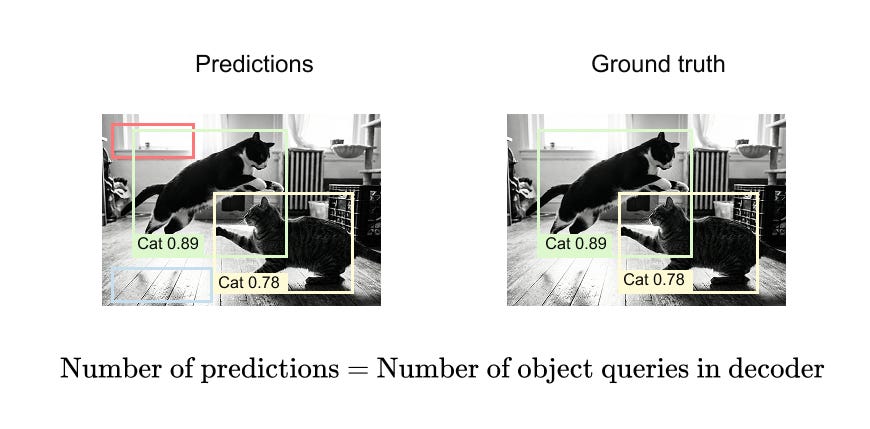
Figure 1.13
Set-based matching between predicted boxes and ground-truth objects using the Hungarian algorithm, with unmatched predictions assigned to background.

1.7 Hungarian Matching Loss in Detection Transformers

Detection Transformers frame object detection as a direct set prediction problem, where a fixed number of predictions must be matched to a variable number of ground-truth objects. Because the predictions are unordered and there is no predefined correspondence between predicted boxes and ground-truth boxes, DETR requires a principled mechanism to establish a one-to-one assignment during training. This role is fulfilled by the Hungarian matching algorithm, which enables global, optimal matching between two sets under a predefined cost.

The Hungarian algorithm originates from the classical assignment problem and provides a deterministic way to compute the minimum-cost matching between two equally sized sets. DETR adopts this algorithm to match predicted object queries to ground-truth objects, ensuring that each object is detected exactly once and that redundant predictions are explicitly penalized.

The Hungarian Algorithm Through the Assignment Problem

To understand Hungarian matching, it is helpful to first consider the classical job assignment problem. Suppose there are four workers and four jobs. Each worker quotes a different cost for performing each job, resulting in a cost matrix where rows represent workers and columns represent jobs. The objective is to assign each worker to exactly one job such that all jobs are completed and the total cost is minimized.

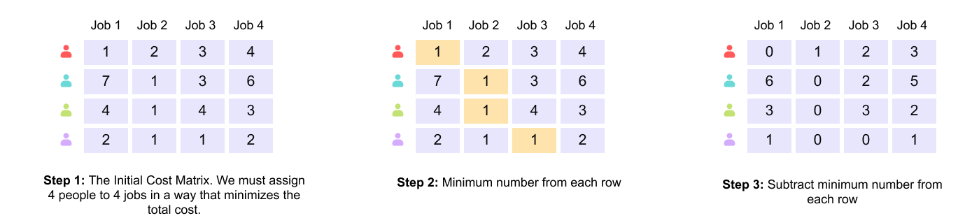
Figure 1.14 Initial cost matrix for the assignment problem, showing the cost quoted by each worker for each job.

In Step 1, the problem is represented as a cost matrix, where each row corresponds to a worker and each column corresponds to a job. The entry at row i, column j denotes the cost incurred if worker i is assigned to job j. The objective is to select exactly one entry from each row and each column such that the total cost is minimized.

In Step 2, the minimum value in each row is identified. This value represents the cheapest job that a particular worker can perform.

In Step 3, the minimum value of each row is subtracted from all elements in that row. This transformation does not change the relative costs between assignments and therefore does not alter the optimal solution. However, it guarantees that every row now contains at least one zero, which simplifies the identification of low-cost assignments.

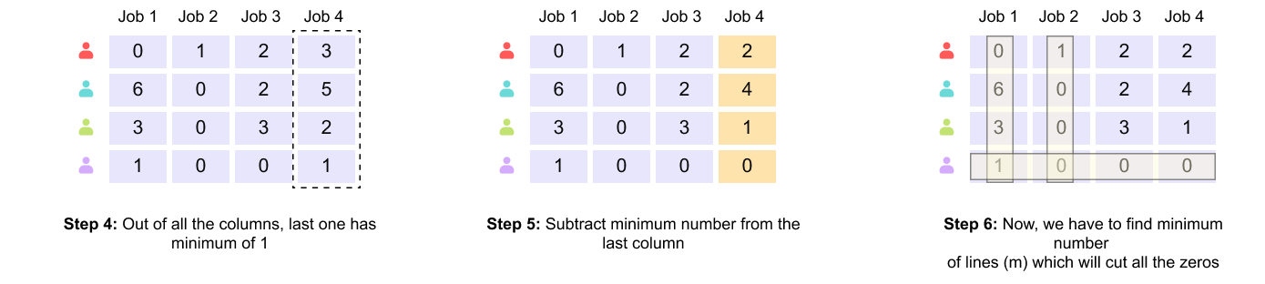
Figure 1.15 Steps 4–6: column-wise normalization and identification of zero structure.

In Step 4, the algorithm inspects each column to determine whether further normalization is required. Columns that already contain a zero are left unchanged.

In Step 5, the minimum value of the last column, which is nonzero, is subtracted from all elements in that column. As with row normalization, this operation preserves the optimal assignment while introducing additional zeros.

In Step 6, the algorithm examines the resulting matrix and prepares to determine whether a complete assignment can be formed using the existing zeros. At this point, the matrix typically contains multiple zeros distributed across rows and columns.

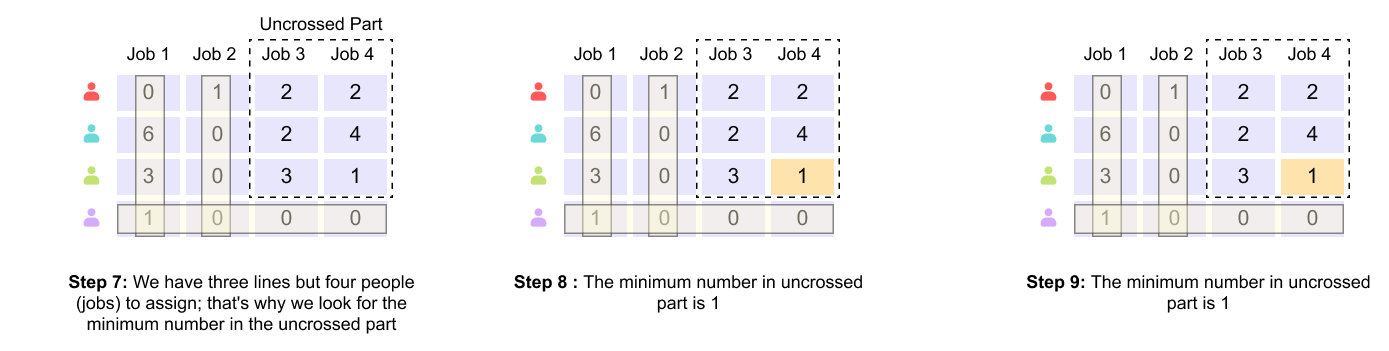
Figure 1.16 Steps 7–9: covering zero entries and identifying the need for further adjustment.

In Step 7, the algorithm attempts to cover all zero entries in the matrix using the minimum number of horizontal and vertical lines. Each line can cover an entire row or column. The key observation here is that the number of lines required is three, while the number of workers and jobs is four.

In Step 8, the algorithm focuses on the uncovered elements, that is, entries not intersected by any line. Among these uncovered elements, the minimum value is identified.

In Step 9, this minimum uncovered value is confirmed. The fact that fewer than four lines are sufficient to cover all zeros indicates that a complete assignment cannot yet be constructed, and the matrix must be adjusted further.

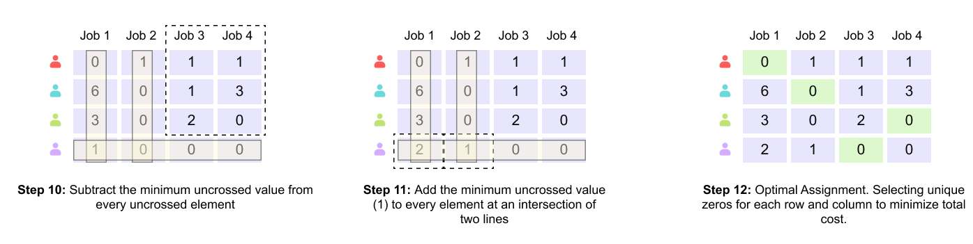
Figure 1.17 Steps 10–12: matrix adjustment and emergence of a complete zero-cost assignment.

In Step 10, the minimum uncovered value is subtracted from every uncovered element. This operation creates new zeros in previously nonzero locations.

In Step 11, the same minimum value is added to every element that lies at the intersection of two covering lines. This compensatory step ensures that no negative values are introduced and that the optimal assignment remains unchanged.

In Step 12, the adjusted matrix now contains a configuration of zeros that allows a unique selection of one zero per row and per column. At this stage, a complete assignment can be constructed.

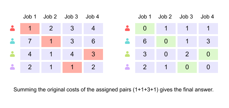
Figure 1.18 Final optimal assignment and recovery of the minimum total cost from the original matrix.

The highlighted zeros correspond to the optimal worker–job pairing. Although the transformed matrix yields a zero total cost, this is an artifact of the normalization process. To recover the true minimum cost, the selected assignments are mapped back to the original cost matrix. Summing the original costs associated with the selected pairs yields the final minimum total cost.

This example illustrates how the Hungarian algorithm converts a global combinatorial optimization problem into a structured sequence of matrix operations. At no point does the algorithm rely on greedy local decisions. Instead, it guarantees a globally optimal one-to-one assignment by systematically reshaping the cost landscape until the optimal solution becomes explicit.

This exact mechanism is later reused in Detection Transformers, where predicted object queries are optimally matched to ground-truth bounding boxes using an analogous cost matrix and the same Hungarian matching procedure.

Figure 1.19 Hungarian matching in DETR, showing one-to-one assignment between predicted bounding boxes and ground-truth objects.

To perform this matching, DETR constructs a cost matrix where each entry represents the cost of assigning a predicted query to a particular ground-truth object. This cost combines classification error and localization error, typically using a weighted sum of class probability loss and bounding box regression terms such as L1 distance and IoU-based loss. Importantly, the cost is computed for all possible pairings, allowing the matching to consider global consistency rather than local heuristics.

Once the optimal assignment is computed using the Hungarian algorithm, the loss is evaluated only on the matched pairs. Predictions assigned to real objects contribute both classification and localization losses, while predictions assigned to the no-object class contribute only a classification loss. This set-based loss formulation ensures that each object is detected exactly once and eliminates the need for non-maximum suppression.

Hungarian matching is not merely a training trick but a foundational component of DETR’s design. By enforcing a global one-to-one correspondence between predictions and ground truth, it removes ambiguity, prevents duplicate detections, and aligns the training objective directly with the final inference output. This shift from heuristic post-processing to principled global optimization is one of the key reasons DETR represents a conceptual departure from traditional object detection pipelines.

1.8 When Hungarian Matching Is Needed and When It Is Not in DETR

Hungarian matching plays a critical role in the training formulation of Detection Transformers, but its use is conditional rather than universal. Whether it is required depends on the structure of the prediction–ground-truth correspondence problem and, in particular, on whether that correspondence is ambiguous.

The simplest case arises when an image contains exactly one ground-truth object. Even though DETR may produce many predictions from multiple object queries, the assignment problem is trivial. Each prediction can be independently compared to the single ground-truth object using a localization cost. The prediction that best matches the ground truth can be selected, and all remaining predictions can be treated as background. Because there is only one object, there is no possibility of conflicting assignments, and no global matching constraint is required.

The situation changes fundamentally once multiple ground-truth objects are present. In this setting, the model must decide not only which predictions are good, but also how to assign them uniquely to different objects. Independent matching decisions are no longer sufficient because they do not enforce exclusivity. A single prediction may appear to be a good match for more than one ground-truth object, leading to ambiguous supervision. Conversely, multiple predictions may compete for the same object, producing unstable and contradictory gradients during training.

Hungarian matching resolves this ambiguity by treating matching as a global optimization problem over sets rather than a collection of independent decisions. DETR constructs a cost matrix between all predictions and all ground-truth objects and computes a one-to-one assignment that minimizes the total cost. Each ground-truth object supervises exactly one prediction, and each prediction is assigned to at most one object. Predictions that are not matched to any ground truth are explicitly treated as background. This set-based formulation is what enables DETR to avoid anchors, heuristics, and non-maximum suppression while still producing stable and well-defined training signals.

In summary, Hungarian matching is unnecessary when the assignment problem is trivial, such as in the single-object case. It becomes essential whenever multiple objects must be matched to multiple predictions in a globally consistent manner.

1.9 The Limitation of IoU and the Motivation for Generalized IoU

Intersection over Union is the most commonly used metric for measuring the overlap between a predicted bounding box and a ground-truth box. It is defined as

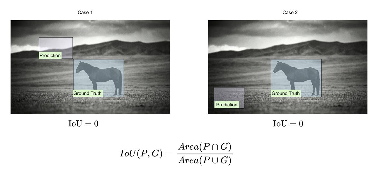
\(\text{IoU}(P, G) = \frac{\text{Area}(P \cap G)}{\text{Area}(P \cup G)}\)

Figure 1.20 Two non-overlapping prediction–ground-truth pairs with identical IoU values of zero. Although one prediction is spatially much closer to the ground truth than the other, IoU fails to distinguish between them.

In both cases shown above, the predicted box does not intersect the ground-truth box, and IoU assigns a value of zero. However, from a learning perspective, the first prediction is clearly better than the second because it is closer to the target. IoU provides no gradient signal that reflects this difference, which leads to poor optimization behavior during training.

To address this limitation, Generalized IoU (GIoU) introduces an additional geometric term that accounts for the distance between boxes. Let C denote the smallest enclosing rectangle that contains both the prediction P and the ground truth G. Generalized IoU is defined as

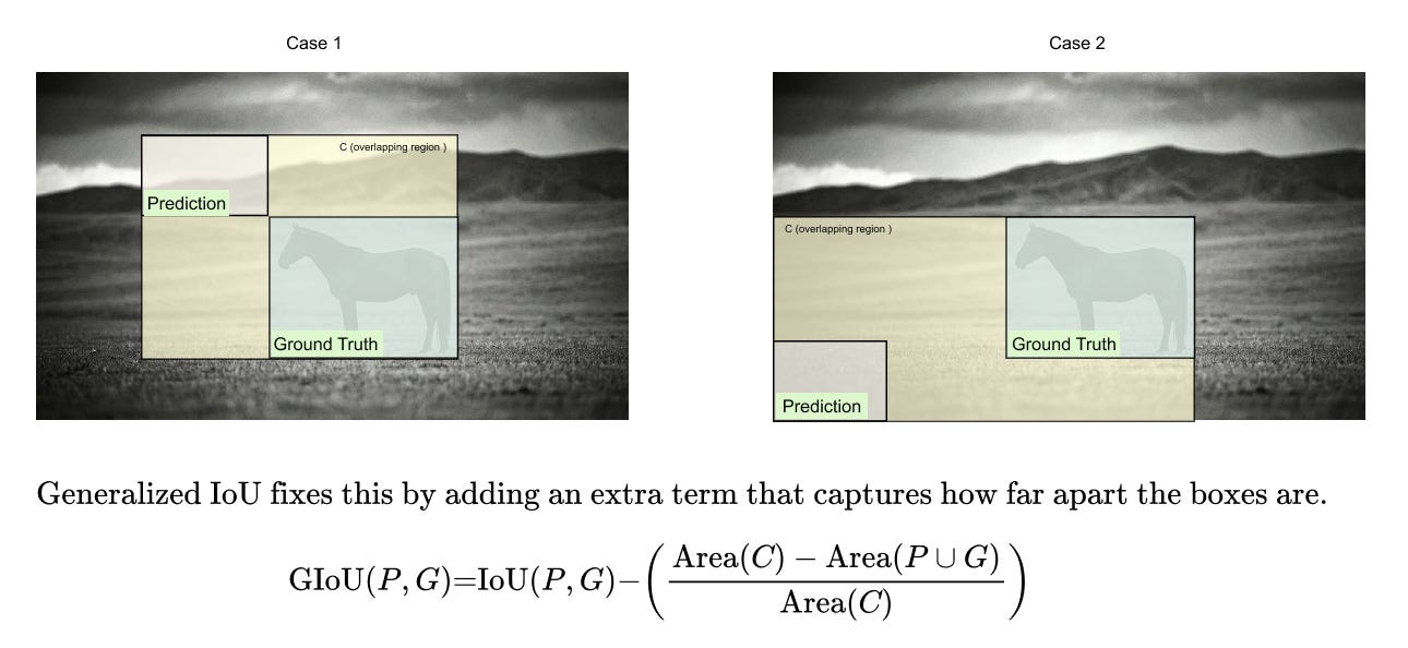
\(\text{GIoU}(P, G) = \text{IoU}(P, G) - \frac{\text{Area}(C) - \text{Area}(P \cup G)}{\text{Area}(C)}\)

Figure 1.21 Generalized IoU introduces the smallest enclosing rectangle C, allowing the metric to penalize predictions that are farther from the ground truth even when there is no overlap.

When IoU is zero, the GIoU expression simplifies to

\(\text{GIoU}(P, G) = -1 + \frac{\text{Area}(P \cup G)}{\text{Area}(C)}\)

If the prediction and ground truth have similar sizes, then Area(P∪G) is approximately constant. The decisive factor becomes Area(C). Predictions that are closer to the ground truth yield a smaller enclosing box C, resulting in a higher GIoU value. In this way, GIoU restores meaningful ordering among non-overlapping predictions and provides a smoother, more informative training signal.

1.10 The DETR Loss Function: Formal Definition and Training Mechanics

The DETR loss is defined over sets rather than ordered lists. Let the model produce a fixed number N of predictions, each consisting of a class probability distribution and a bounding box. Let the ground truth consist of M objects, where M ≤ N. To construct a square matching problem, the ground truth is augmented with N−M null objects.

Hungarian Matching

DETR first computes a cost matrix between all predictions and all ground-truth objects. The cost for matching prediction i with ground-truth object j is defined as

\(\mathcal{C}_{ij} = \lambda_{\text{cls}} \mathcal{L}_{\text{cls}}(i, j) + \lambda_{L1} \|b_i - b_j\|_1 + \lambda_{\text{GIoU}} \mathcal{L}_{\text{GIoU}}(b_i, b_j)\)

where L_cls is the classification loss, b_i = (x,y,w,h) denotes the predicted box and b_j denotes the ground-truth box

The Hungarian algorithm finds the permutation σ that minimizes the total matching cost

\(\sigma^* = \arg \min_{\sigma} \sum_{j=1}^{N} \mathcal{C}_{\sigma(j),j}\)

Final Loss

Once the optimal assignment is computed, the final DETR loss is defined as

\(\mathcal{L} = \sum_{j=1}^{N} \left[ \mathcal{L}_{\text{cls}}(\hat{c}_{\sigma^*(j)}, c_j) + \mathbb{1}_{\{c_j \neq \varnothing\}} \left( \lambda_{L1} \|b_{\sigma^*(j)} - b_j\|_1 + \lambda_{\text{GIoU}} \mathcal{L}_{\text{GIoU}}(b_{\sigma^*(j)}, b_j) \right) \right]\)

Localization losses are applied only to matched non-null objects, while unmatched predictions are trained purely through the classification loss as background.

An important implementation detail is that DETR applies this loss not only to the final decoder layer, but also to intermediate decoder outputs during training. These auxiliary losses improve gradient flow and stabilize optimization. During inference, only the final decoder output is used.

1.11 Concluding Perspective on DETR

Detection Transformers represent a conceptual shift in object detection. Instead of framing detection as a dense prediction problem with anchors, heuristics, and post-processing, DETR formulates detection as a set prediction problem. Object queries act as slots that compete to explain the objects present in an image, and Hungarian matching provides the mathematical mechanism that enforces a clean, one-to-one correspondence between predictions and ground truth.

This design eliminates the need for non-maximum suppression, anchor tuning, and hand-crafted assignment rules. At the same time, it demands careful loss design, robust geometric metrics such as Generalized IoU, and global optimization during training.

Although the original DETR model is computationally expensive and slow to converge, its formulation has influenced an entire family of transformer-based detectors. The core ideas of set-based prediction, bipartite matching, and global supervision continue to shape modern object detection architectures and provide a clean conceptual foundation for unifying detection with broader multimodal and sequence modeling frameworks

Watch the full lecture video here

If you would like to deepen your understanding of Detection Transformer and see these ideas explained visually and intuitively, you can refer to the accompanying video linked above. If you wish to get access to our code files, handwritten notes, all lecture videos, Discord channel, and other PDF handbooks that we have compiled, along with a code certificate at the end of the program, you can consider being part of the pro version of the “Transformers for Vision Bootcamp”. You will find the details here:

https://vision-transformer.vizuara.ai/