Coding a Vision Transformer (almost) from scratch

Using PyTorch in 100 minutes

and

Jul 17, 2025

There is something special about deep, uninterrupted work. The kind of session where you forget your phone exists, the world outside quiets down, and your mind latches onto a single idea with complete focus. Last week, I gave myself a challenge: build a Vision Transformer from scratch using PyTorch. No pre-trained models. No high-level libraries. No AI assistants.

Just me, a blank Colab notebook, and the MNIST dataset.

It was a four-hour stretch of pure concentration. I had no intention of making it a lecture, but as I started explaining my own thoughts aloud while coding, I realized this could be a great learning resource. So I hit record. What came out was a 100-minute walkthrough, where I not only built a working ViT from scratch, but also explained every line, every component, and every idea behind it.

This article captures the essence of that session.

Why Vision Transformers?

When transformers first arrived in 2017 through the "Attention is All You Need" paper, they reshaped the field of natural language processing. Three years later, Google researchers extended those ideas to images and introduced the Vision Transformer. Instead of feeding in sequences of words, the model processes sequences of image patches. It sounds simple enough. But the architectural shift is profound.

CNNs operate with a strong inductive bias toward locality and translation invariance. Transformers, on the other hand, treat the image as a set of flat patches and let self-attention learn the spatial relationships. There are no convolutions, no pooling layers. Just attention and projection.

I have used transformers in the past, but never wrote one for vision tasks from scratch. That felt like a gap worth filling.

The Architecture, Explained for Humans

Before diving into code, I spent the first part of the lecture walking through the ViT architecture in plain language.

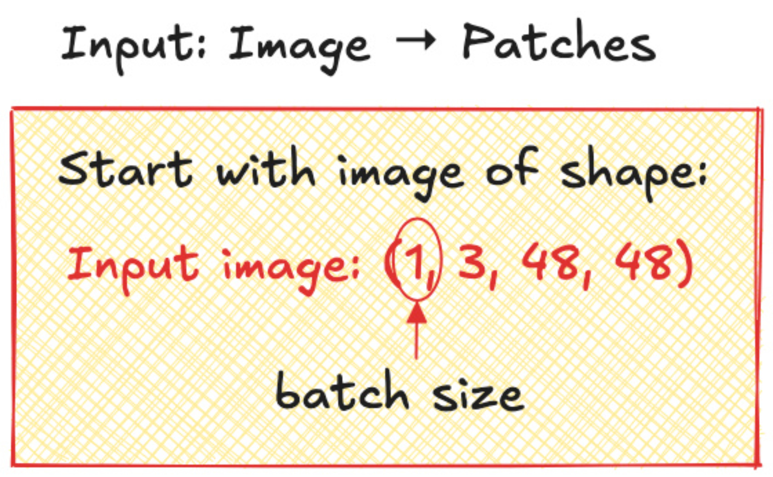
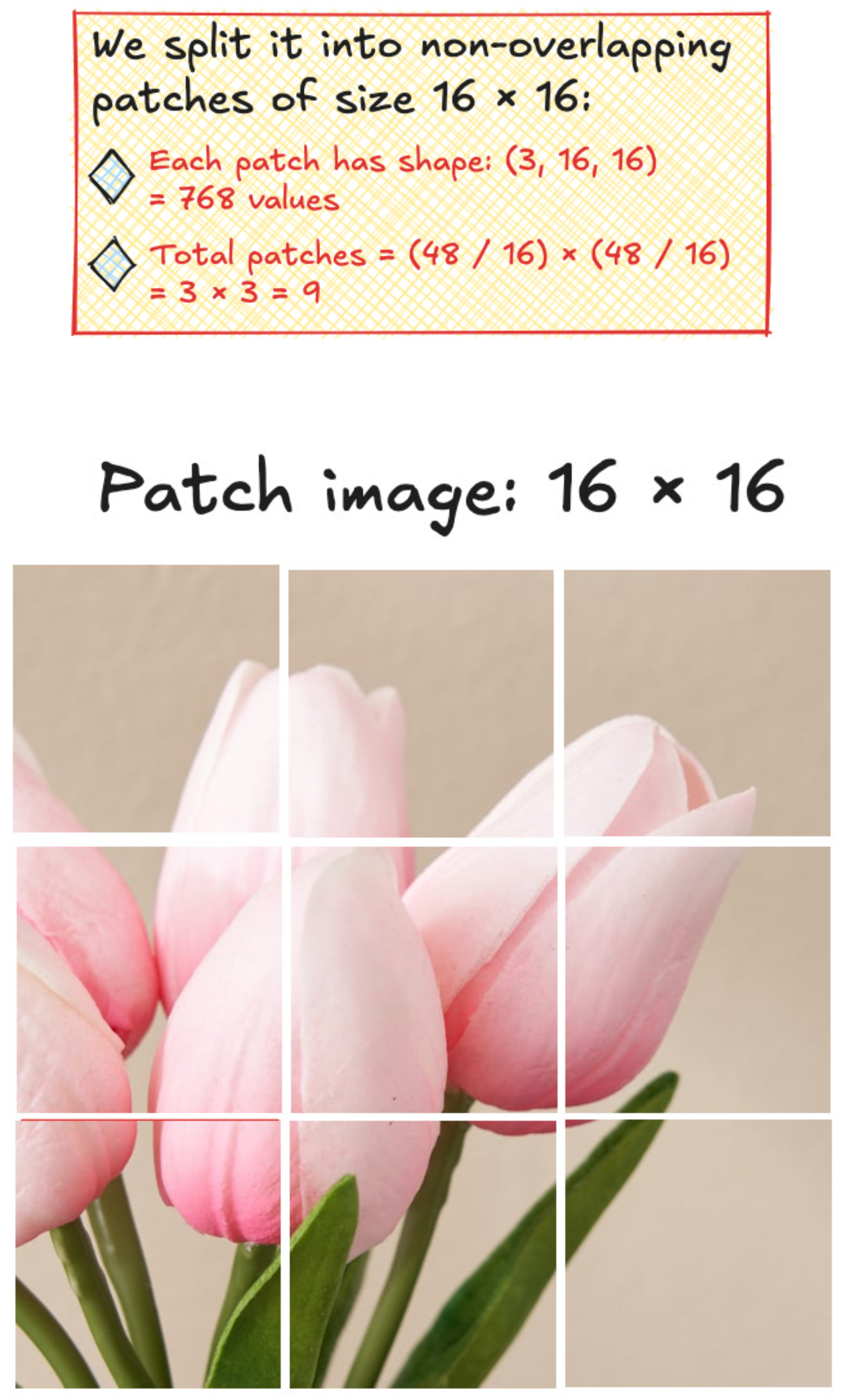
An image is divided into patches, like 16x16 squares. Each patch is then flattened and projected into a vector of fixed dimension - say, 768. Just as a sentence in NLP becomes a sequence of word embeddings, the image becomes a sequence of patch embeddings.

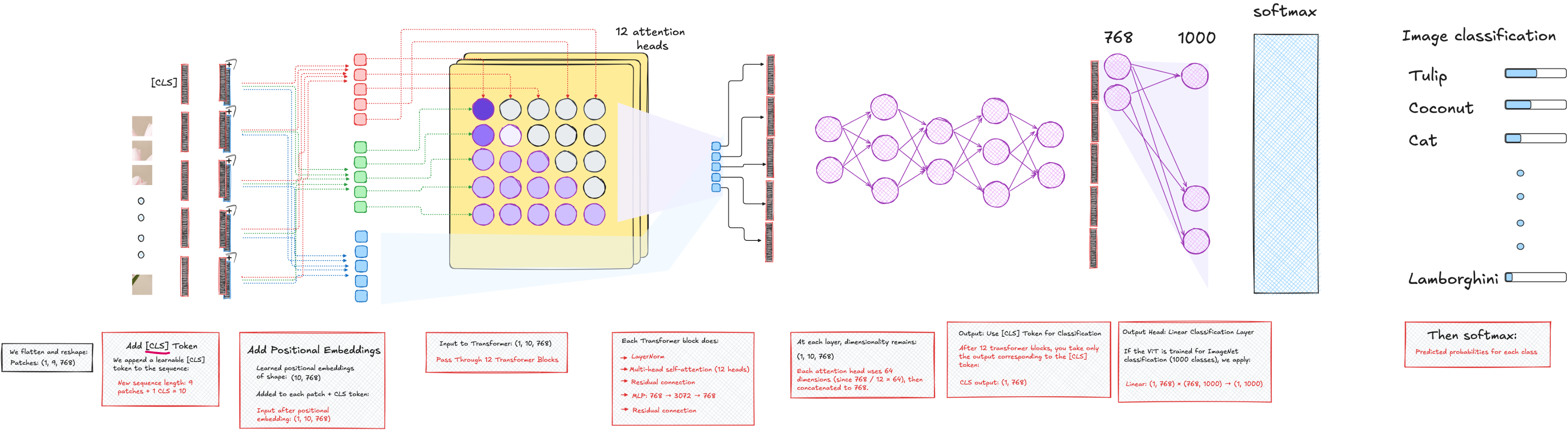
To this sequence, we prepend a learnable vector called the CLS token. Its job is to absorb the information across the entire image, and eventually act as the representation used for classification. We also add positional encodings to each patch embedding, so the model can retain information about spatial order.

The resulting sequence is then fed into a transformer encoder. Each encoder block consists of multi-head attention, layer normalization, residual connections, and an MLP. After several such blocks, we extract the CLS token and pass it through another MLP head to perform classification.

In our case, the goal was to classify MNIST digits, so the final output layer had 10 dimensions.

That is the entire pipeline, but it hides many details. So let me walk you through how I implemented it.

From blank notebook to working code

I began by defining the patch embedding module. Instead of writing a custom patch extraction routine, I used a 2D convolution layer with kernel size and stride equal to the patch size. This effectively slices the image into non-overlapping patches and maps each to a learnable embedding.

After the convolution, I flattened the spatial dimensions and transposed the tensor so that it had shape [batch_size, num_patches, embed_dim]. This format is essential because PyTorch's multi-head attention layer expects the batch to come first when using batch_first=True.

#import required libraries
import torch
import torchvision
import matplotlib.pyplot as plt
import torchvision.transforms as transforms
import torch.utils.data as dataloader
import torch.nn as nn

#transformation of PIL data into tensor format
transformation_operation = transforms.Compose([transforms.ToTensor()])

#getting PIL data
train_dataset = torchvision.datasets.MNIST(root='./data', train=True, download=True, transform = transformation_operation)
val_dataset = torchvision.datasets.MNIST(root='./data', train=False, download=True, transform = transformation_operation)

#define variables
batch_size = 64
num_classes = 10
num_channels = 1
img_size = 28
patch_size = 7
patch_num = (img_size // patch_size) * (img_size // patch_size)
attention_heads = 1
embed_dim = 16
transformer_blocks = 1
mlp_nodes = 16
learning_rate = 0.01
epochs = 5

#using dataloader to prepare data for the neural network
train_data = dataloader.DataLoader(train_dataset, shuffle = True, batch_size = batch_size)
val_data = dataloader.DataLoader(val_dataset, shuffle = True, batch_size = batch_size)

Next, I initialized the CLS token as a learnable parameter with shape [1, 1, embed_dim], and the positional embedding as [1, num_patches + 1, embed_dim]. I ensured both were registered properly so that they would be updated during training.

#class for PatchEmbedding - Part 1 of the ViT architecture

class PatchEmbedding(nn.Module):
    def __init__(self):
        super().__init__()
        self.patch_embed = nn.Conv2d(num_channels, embed_dim, kernel_size= patch_size, stride = patch_size )

    def forward(self, x):
        x = self.patch_embed(x)
        x = x.flatten(2)
        x = x.transpose(1,2)
        return x

Then came the transformer encoder. I wrote a class with two layer normalizations, one multi-head attention layer, and an MLP. The MLP increased the embedding size to a higher dimension and then brought it back to the original size, with a GELU activation in between. Residual connections wrapped both the attention and MLP components.

class TransformerEncoder(nn.Module):
    def __init__(self):
        super().__init__()
        self.layer_norm1 = nn.LayerNorm(embed_dim)
        self.multi_head_attention = nn.MultiheadAttention(embed_dim, attention_heads, batch_first=True)
        self.layer_norm2 = nn.LayerNorm(embed_dim)
        self.mlp = nn.Sequential(
            nn.Linear(embed_dim,mlp_nodes),
            nn.GELU(),
            nn.Linear(mlp_nodes,embed_dim)

        )

    def forward(self, x):
        residual1 = x
        x = self.layer_norm1(x)
        x = self.multi_head_attention(x, x, x)[0] + residual1
        residual2 = x
        x = self.layer_norm2(x)
        x = self.mlp(x) + residual2
        return x

I repeated the transformer encoder block multiple times using a loop wrapped in nn.Sequential, allowing easy variation of the depth.

#class for MLP head for classification - Part 3 of the ViT architecture
class MLP_Head(nn.Module):
    def __init__(self):
        super().__init__()
        self.layernorm3 = nn.LayerNorm(embed_dim)
        self.mlphead = nn.Sequential(
            # nn.LayerNorm(embed_dim),
            nn.Linear(embed_dim, num_classes)
        )

    def forward(self, x):
        # x = x[:,0]
        x = self.layernorm3(x)
        x = self.mlphead(x)
        return x

The final component was the MLP head for classification. This took only the CLS token (the first vector in the sequence) and passed it through a linear layer that mapped to 10 output classes. Optionally, I added a layer normalization here as well.

Putting it all together, I built a VisionTransformer class that composed the patch embedding, CLS and positional tokens, transformer blocks, and classification head.

class VisionTransformer(nn.Module):
    def __init__(self):
        super().__init__()
        self.patch_embedding = PatchEmbedding()
        self.cls_token = nn.Parameter(torch.randn(1,1,embed_dim))
        self.position_embedding = nn.Parameter(torch.randn(1,patch_num+1,embed_dim))
        self.transformer_blocks = nn.Sequential(*[TransformerEncoder() for _ in range (transformer_blocks)])
        self.mlp_head = MLP_Head()

    def forward(self,x):
        x = self.patch_embedding(x)
        B = x.size(0)
        cls_tokens = self.cls_token.expand(B,-1,-1)
        x = torch.cat((cls_tokens,x),1)
        x = x + self.position_embedding
        x = self.transformer_blocks(x)
        x = x[:,0]
        x = self.mlp_head(x)
        return x

Training on MNIST

Once the model was ready, I loaded the MNIST dataset using torchvision.datasets.MNIST. I used basic tensor transformations and defined a simple dataloader with batch size 64.

#device
#optimizer
#crossentropy

device = torch.device("cuda:0" if torch.cuda.is_available() else "cpu")
model = VisionTransformer().to(device)

optimizer = torch.optim.Adam(model.parameters(), lr = learning_rate)
criterion = nn.CrossEntropyLoss()

The training loop followed the usual pattern: forward pass, compute loss, backward pass, and update parameters. I used the Adam optimizer and cross-entropy loss. Initially, the accuracy hovered around 10 percent, which was expected due to random initialization.

for epoch in range(5):
    model.train()
    total_loss = 0
    correct_epoch = 0
    total_epoch = 0
    print(f"\nEpoch {epoch+1}")

    for batch_idx, (images, labels) in enumerate(train_data):
        images, labels = images.to(device), labels.to(device)
        optimizer.zero_grad()
        outputs = model(images)

        loss = criterion(outputs, labels)
        loss.backward()
        optimizer.step()

        total_loss+=loss.item()
        preds = outputs.argmax(dim=1)

        correct = (preds == labels).sum().item()
        accuracy = 100.0 * correct / labels.size(0)

        correct_epoch += correct
        total_epoch += labels.size(0)

        if batch_idx % 100 == 0:
            print(f"  Batch {batch_idx+1:3d}: Loss = {loss.item():.4f}, Accuracy = {accuracy:.2f}%")

    epoch_acc = 100.0 * correct_epoch / total_epoch
    print(f"==> Epoch {epoch+1} Summary: Total Loss = {total_loss:.4f}, Accuracy = {epoch_acc:.2f}%")

But once I fixed a critical bug - setting batch_first=True in the multi-head attention - the model began learning rapidly. After five epochs, it reached 96 percent accuracy on the training and validation sets.

I also experimented with reducing the number of attention heads and transformer blocks. Even with a single-head, single-block setup, the model achieved 80 percent accuracy. That is quite remarkable, considering the minimal setup and small dataset.

Lessons and reflections

The entire process reinforced something I often tell students: you do not really understand a model until you implement it yourself. Reading the ViT paper is useful. Using HuggingFace models is convenient. But building a transformer from the ground up forces you to grapple with every design choice.

I also realized how approachable transformers can be, once broken down into their components. The architecture is modular and elegant. PyTorch’s support for things like multi-head attention and layer normalization makes it even easier to experiment.

More importantly, it reminded me that deep work still matters. I did not context switch. I did not reach for quick fixes. I just sat down and focused. And that focus turned into something I am proud of.

If you are learning about transformers or trying to go beyond the surface-level tutorials, I highly recommend doing this exercise. Take a small dataset, write every line yourself, and observe what happens. It will change the way you understand these models.

I have shared the full Colab notebook and the video lecture, where I walk through every concept and line of code. It is long, but if you follow along, I believe it will give you a strong mental model of how Vision Transformers really work.

Thanks for reading. And more importantly, thanks for building.