
Classical filters & convolution: The heart of computer vision
Simple math, profound utility


Before Deep Learning exploded onto the scene, traditional computer vision centered on filters. Filters were small, hand-engineered matrices that you convolved with an image to detect specific features like edges, corners, or textures. In this article, we will dive into the details of classical filters and convolution operation - how they work, why they matter, and how to implement them.

Image filter and convolution
In the simplest sense, an image filter (often called a kernel) is a small matrix that you place over an image (pixel by pixel) to produce some transformation.
For each pixel, you:
Overlay the filter on the local neighborhood of that pixel (commonly a 3×3 or 5×5 region).
Multiply each filter entry by the corresponding pixel intensity.
Sum all these products to produce a single new intensity (or gradient value, or some other measure).
The below image is an example of convolution operation using a 3x3 filter applied on a 5x5 matrix.

This process is called convolution (more precisely, cross-correlation if we don’t rotate the kernel, but in most computer-vision libraries, we call it convolution for simplicity).
Why use filters?
Filters can perform the following operations, making them very useful in image processing.
Feature extraction: To detect edges, corners, or textures (brick walls, repetitive patterns), filters help highlight specific regions.
Noise reduction: Smoothing filters like Gaussian blur can suppress pixel-level noise.
Enhancement: Some filters sharpen or enhance edges to make further analysis (like object segmentation) more robust.
Classical pattern recognition: Long before neural networks, many CV tasks (face detection, license plate recognition) involved carefully chosen filters plus rule-based heuristics.
The below image is a vertical left edge detection filter applied on the famous MNIST hand written image.

In this article, we will discuss about various famous filters. But, instead of directly jumping into them, let us try to logically construct some filters ourselves.
Let us try to logically build some filters
Whenever you see a filter like this:

…it is natural to wonder: Why those numbers? Where did they come from?
Classic filters (like Sobel, Prewitt, Laplacian, etc.) didn’t just pop up out of thin air.
They come from a mix of mathematical foundations (finite differences, derivatives, smoothing) and practical experiments with real images.
Let us go under the hood and see how these shapes and values emerged.
The core idea: Approximating derivatives in 2D
In calculus, an edge is basically a place where the intensity function of an image changes abruptly.
Mathematically, that is a derivative - a measure of how fast a function f(x) is changing. For an image whose pixel values can be described as I(x,y), you have partial derivatives ∂I/∂x (change in the x-direction) and ∂I/∂y (change in the y-direction).
In a digital image, we don’t have continuous functions but discrete pixels. Hence, we approximate derivatives using finite differences.
Simple 1D finite difference
If you want to approximate the derivative d/dx of a function f at a point x, you can do:

Why? Because if you imagine the function as a sequence of values, the difference between neighbors can represent how fast the function is changing.
Translating finite differences to to 2D
For images, we do something similar in both the x and y directions. A very simple gradient filter for the x-direction might look like:
That is the simplest finite difference: pixel to the right minus pixel to the left.
But real images have noise and require more stable computations, so we tweak these simple differences into more sophisticated filters (like Sobel or Prewitt) - we will discuss these filters in detail.
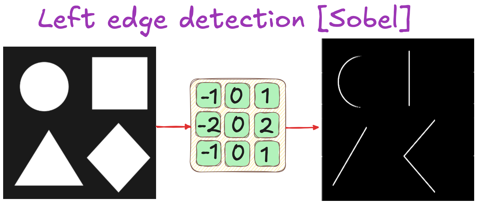
Sobel filter
Sobel is essentially a discrete approximation of the first derivative in x and y directions, plus a bit of smoothing to reduce noise. Its vertical kernel (filter) is:

Why particularly this matrix?
“Smoothing” + “differentiation”
The middle column (all zeros) is for computing the difference in x-direction. If you sum the left column’s values, you get −1+−2+−1=−4. The right column’s values sum to 1+2+1=4. This difference (left vs. right) approximates how big the change is along the x-axis.
Notice the bigger weight in the middle row (−2 and 2)? This is a “smoother” finite difference, giving extra weight to the center row. It helps suppress noise that might exist at the top or bottom rows of the 3×3 patch.
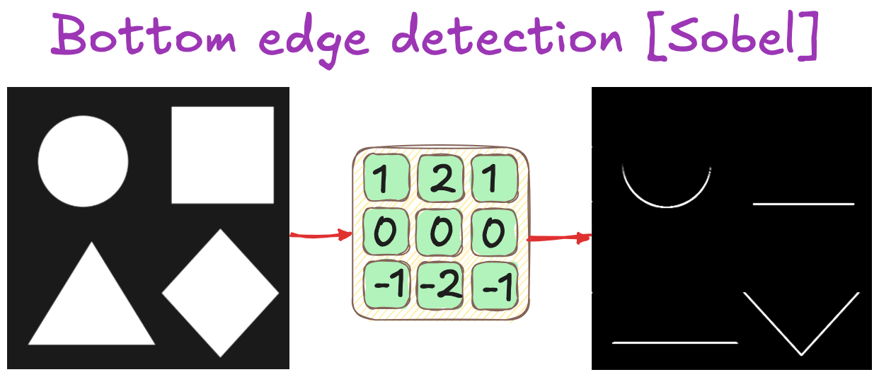
When you convolve an image with this Sobel kernel, you get an approximation of ∂I/∂x. You get the y-direction filter for calculating ∂I/∂x by rotating or by using a transposed version as shown below:

Why is [−1,−2,−1] “smoother” than [-1,1]?
In simple finite-difference filters (e.g., [−1,1] for a 1D gradient), you are only comparing two adjacent pixels. That comparison is extremely direct and thus very sensitive to noise in either pixel.
When you move to something like [−1,0,1] or, more specifically, [−1,−2,−1] vs. [1,2,1] in the Sobel kernel, you are effectively averaging across three pixels (top, center, bottom or left, center, right). By giving a larger weight (e.g., ±2) to the center row or column, the filter collects information from a wider local area and hence “smooths” out the contribution from any single noisy pixel.
In other words:
[−1,1] directly measures the difference of immediate neighbors. Noise in either pixel is fully reflected in the gradient value.
[−1,−2,−1] and [1,2,1] (for Sobel) spreads the gradient calculation across multiple pixels, weighting the center row more. This increased neighborhood sampling and weighting is why it is considered “smoother” and typically more robust to noise.
So why not a simpler filter?
You could do something like:

But that is extremely sensitive to noise. The Sobel’s extra weighting in the center row and its 3×3 size both make the gradient estimate smoother and more robust.
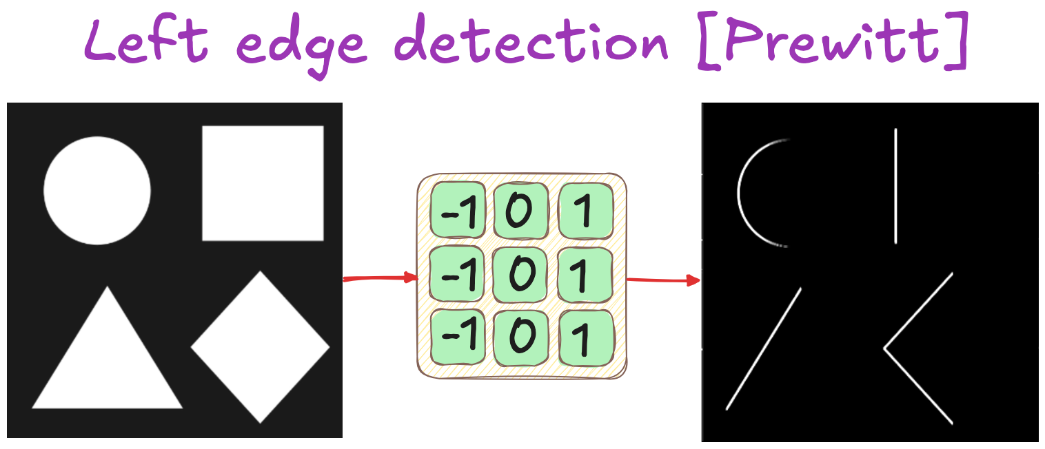
Prewitt filter: A simplified alternative to Sobel
Prewitt is basically the same concept as Sobel - finite difference plus a small smoothing component - but the weights are simpler integers. For vertical edges:

No doubling in the center row - just a uniform weighting of −1 on one side and +1 on the other. In practice, Sobel is sometimes preferred due to slightly better smoothing. But Prewitt still does a decent job and is mathematically straightforward.
Laplacian filter: Second derivative
Edges often become even clearer when you look at the second derivative of an image. The second derivative amplifies rapid intensity changes more aggressively than the first derivative. It essentially looks for how fast the gradient itself is changing. This often produces sharper “peaks” (or zero-crossings) precisely at edges, making them appear more distinct in a second-derivative map.

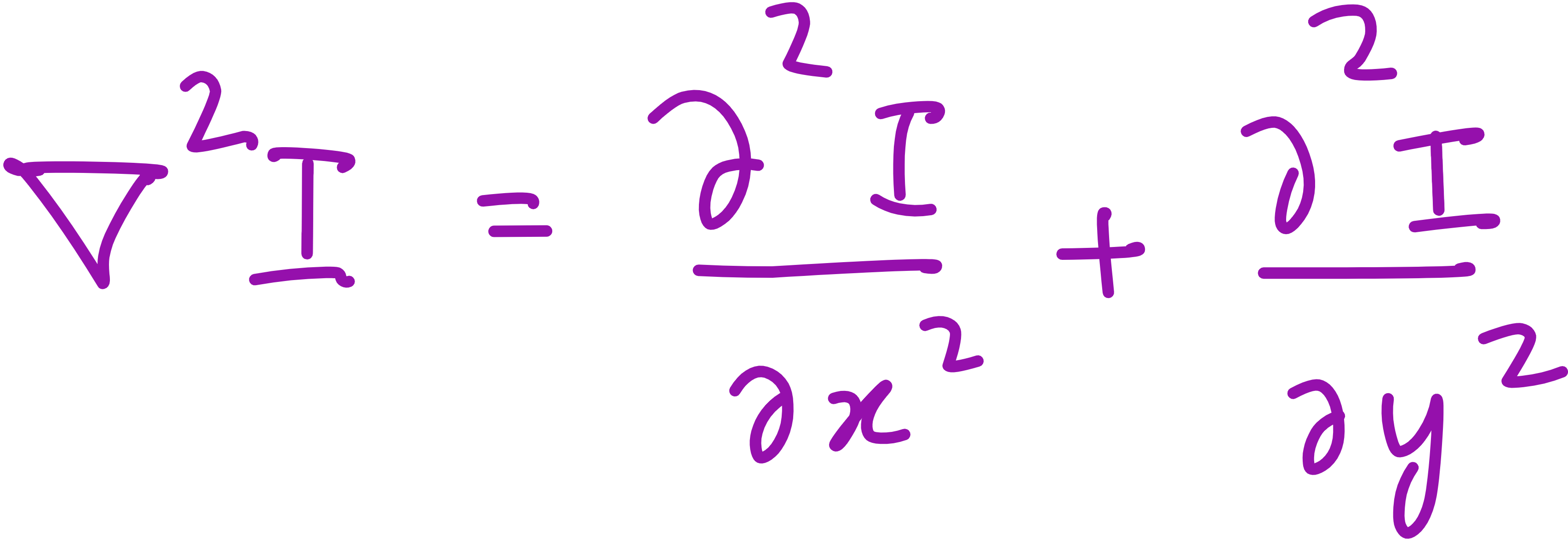
At the heart of the Laplacian operator lies one core principle: it highlights where intensity changes rapidly in all directions. In mathematics, the Laplacian is a second-derivative operation that, in continuous form, looks like:
The Laplacian operator filter is basically:

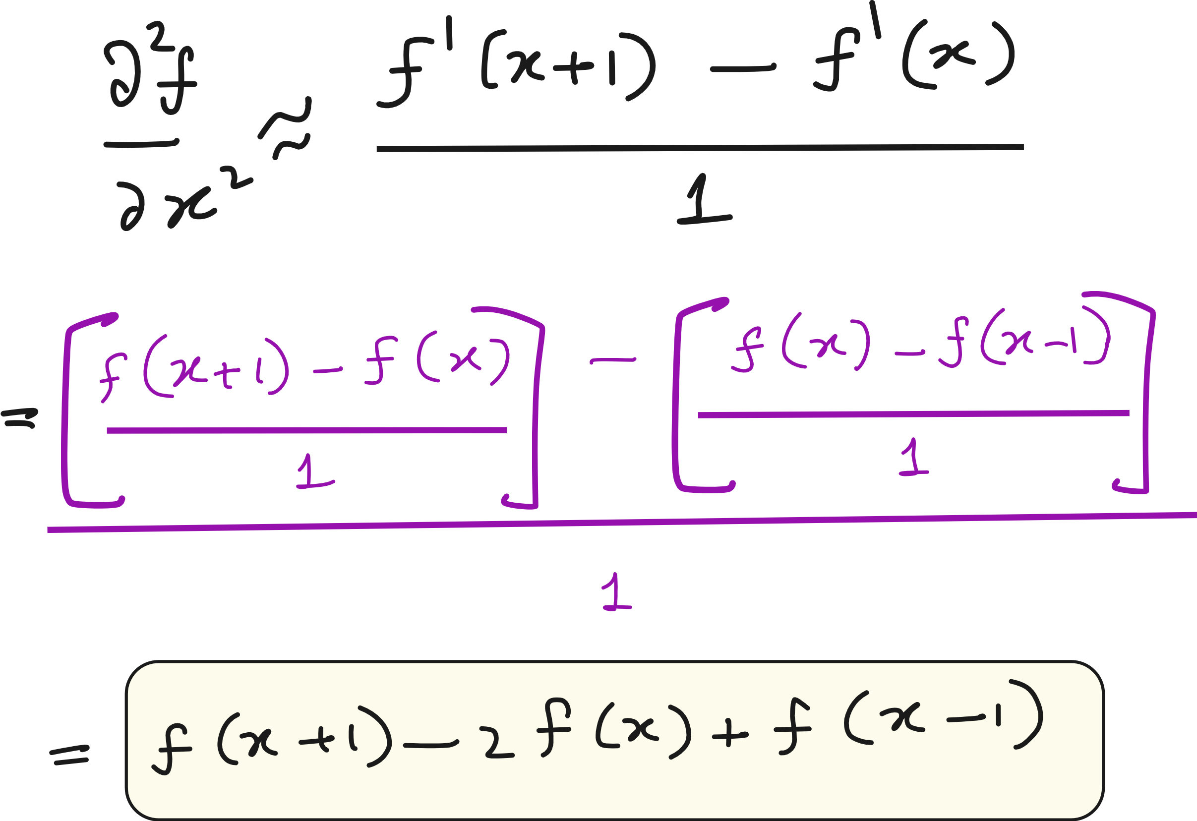
The Laplacian kernel shown above isn’t random. It is a direct outcome of taking the second derivative in both x and y directions in a discrete image. Numerically, it corresponds to summing the four direct neighbors (top, bottom, left, right) and subtracting 4 times the center pixel.
An edge in an image is where brightness values shift quickly from dark to light (or vice versa). The Laplacian operator emphasizes these transitions, often creating strong responses exactly where the intensity changes fastest.
The logic of negative center, positive neighbors
The middle pixel has a large negative value (−4). This is equivalent to subtracting the “average” intensity around it.
Neighboring pixels each have a smaller positive weight. This highlights places where there’s a rapid change in intensity (the hallmark of edges).
The Laplacian kernel isn’t random: it’s a direct outcome of taking the second derivative in both x and y directions in a discrete image. Numerically, it corresponds to summing the four direct neighbors (top, bottom, left, right) and subtracting 4 times the center pixel:

Why do some filters look symmetrical?
Symmetry ensures:
Balanced response: Negative weights on one side, positive on the other (like −1,1 or −2,2).
No directional bias: The filter picks up changes in the same way if you move left-to-right or right-to-left.
Less shifting: A symmetrical kernel won’t shift features in the resulting image.
Let us play with some kernels
Consider this image.

Say we want to construct filters for the following operations.
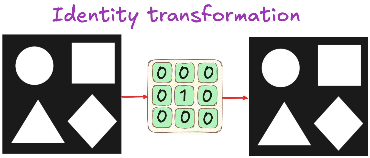
Identity transformation (no change to the image)
Top edges detection
Bottom edges detection
Right edges detection
Left edges detection
Slanted edge detection
Outline (edge) detection
Blurring the image
Denoising
The following filters allow the above operations. You can play with the values of filters and see what happens to your input image here: https://setosa.io/ev/image-kernels/


Filters: Historical & practical considerations
Finite-Difference Approximations (1960s+): Early researchers realized that edges in images correspond to large intensity changes. The discrete derivative is the simplest way to measure that.
Noise: Real images are noisy, so a naive approach (like
[ -1, 1 ]) was too sensitive. Researchers added smoothing to the kernel shape. That’s how we got kernels like Sobel.Computational Resources: In older systems with limited CPU power, a 3×3 filter was a compact way to approximate derivatives without requiring big memory or advanced hardware.
Empirical Fine-Tuning: Even with the math, early computer vision scientists would experiment on actual images—adjusting the kernel’s center or corners until it performed well on edge tasks.
Summary: The “shape” is not arbitrary
Derivatives: The difference-based approach to detect changes.
Smoothing: Additional coefficients (like ±2) reduce noise.
Symmetry: Helps keep the filter balanced.
Practical Tuning: Some constants (−1,1- or −1,0, or −2,0) arise from a combination of math and real-world testing.
So the next time you look at a 3×3 edge-detection kernel, remember: it is basically a discrete derivative plus some smoothing. Its sign pattern and numeric weights encode the essential logic of how to highlight intensity changes (edges) or second-derivative changes (Laplacian).
Additional resources to check out for visualizing filters and convolution operation
https://deeplizard.com/resource/pavq7noze2
https://ezyang.github.io/convolution-visualizer/
Lecture video
I have released a lecture video on this topic on Vizuara’s YouTube channel. Do check this out. I hope you enjoy watching this lecture as much as I enjoyed making it.