
Building a Nano Vision-Language Model from Scratch


Vision–Language Models (VLMs) form the foundation of modern multimodal artificial intelligence. They allow machines to understand images and text not as separate modalities, but as concepts that occupy a common semantic space. Models such as CLIP (Contrastive Language–Image Pre-training) demonstrated that aligning text and image representations enables robust performance in tasks like retrieval, captioning, and zero-shot classification.
Most existing explanations of VLMs either remain abstract or focus only on usage of pre-trained models. In contrast, this article reconstructs the fundamentals of a VLM from the beginning by building a compact or “nano” version of a CLIP-style model. The intention is not to compete with large models, but to understand the internal mechanisms of dataset creation, dual encoders, joint embedding space, and contrastive training.
1. Problem Definition
The core task for the nano-VLM is retrieval. Given an input caption, the model should select the best matching image from a set of candidate images. Conversely, given an image, it should retrieve the correct caption. For this, the model must encode both modalities into a common embedding space such that related image–text pairs lie close to each other, while unrelated pairs remain far apart.
This is fundamentally different from classification tasks. In image classification, a single label is shared among many images. Here, each image has a unique caption, and the model must learn to represent fine-grained attributes such as colour, shape, and spatial position.
2. Synthetic Dataset Construction
Instead of using large datasets like COCO or Flickr30k, a simple yet complete synthetic dataset is programmatically generated. This has several advantages: complete control over data attributes, ability to understand each image–caption pair precisely, and low computational requirements.
The dataset is constructed using three elements:
Shapes: circle, square, triangle
Colours: nine in total (for example, red, green, blue, yellow, pink, brown, etc.)
Positions: nine positions inside the image grid – top, bottom, left, right, centre, and the four corners
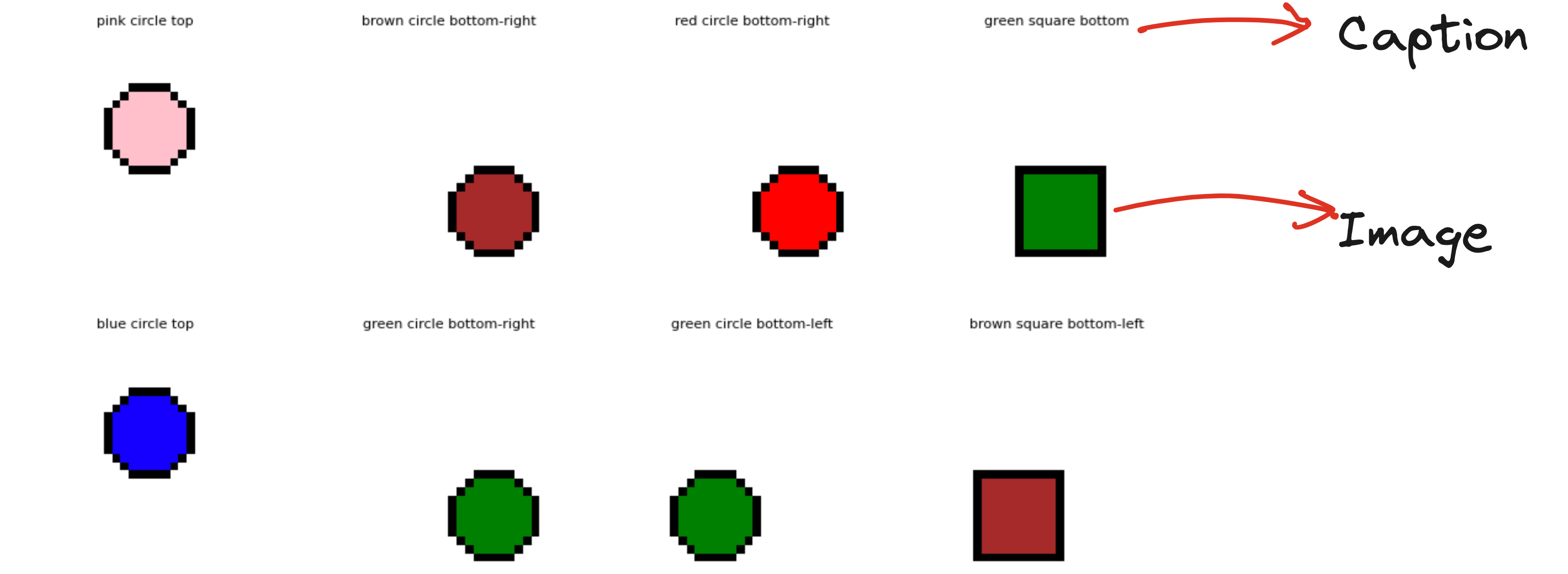
The total number of unique captions is:
9 colours × 3 shapes × 9 positions = 243 image–caption pairs
Each image is a 32×32 RGB canvas generated using the Python PIL library. Shapes are drawn within a defined margin so they do not touch the image boundary.
A caption follows the structure:<colour> <shape> <position>
For example: pink circle top, green square bottom-right
These captions serve as natural language descriptions instead of categorical labels.
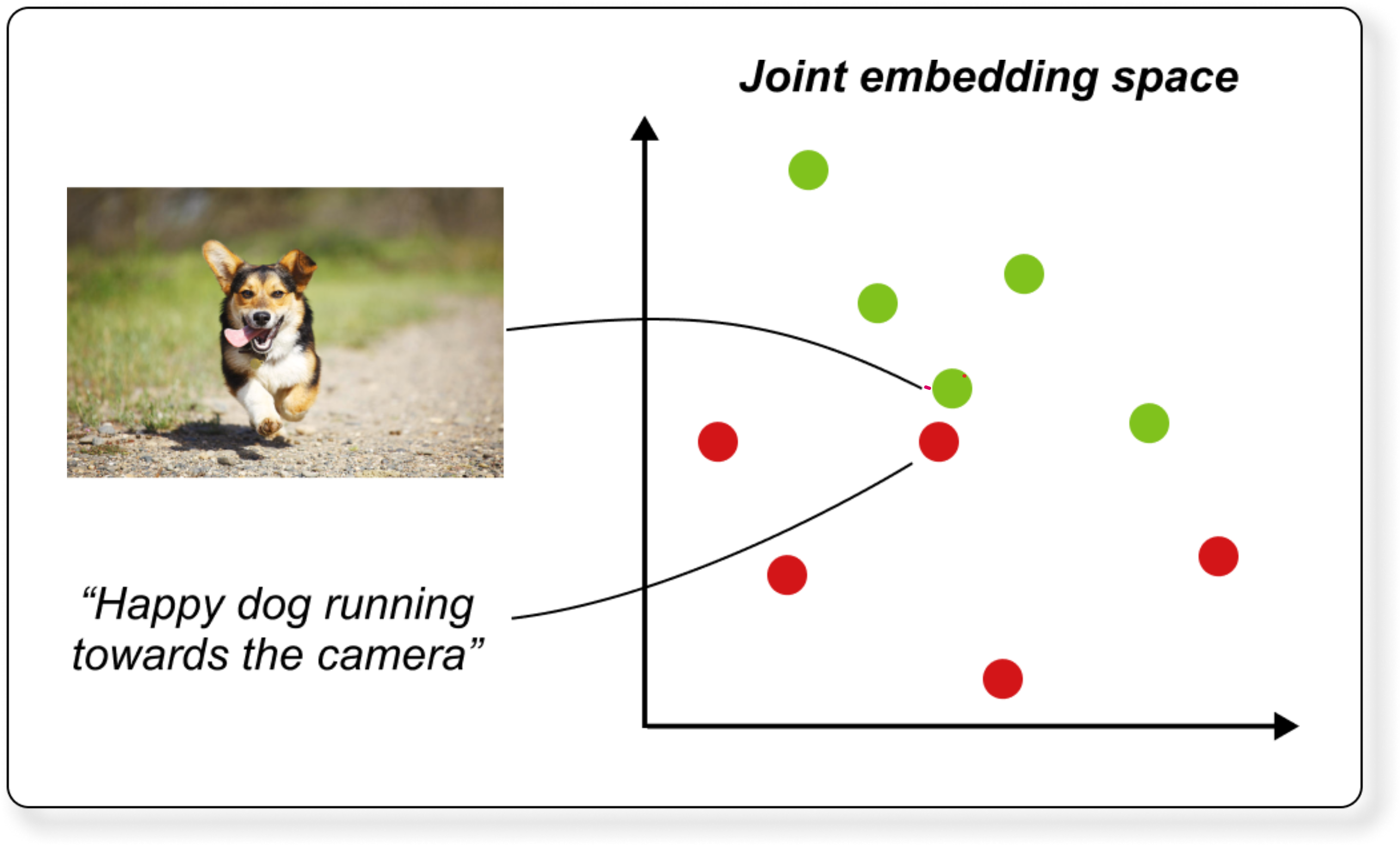
3. Joint Embedding Space
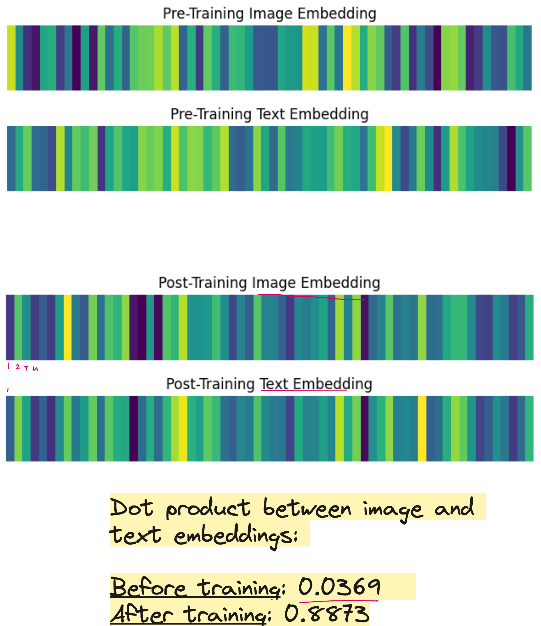
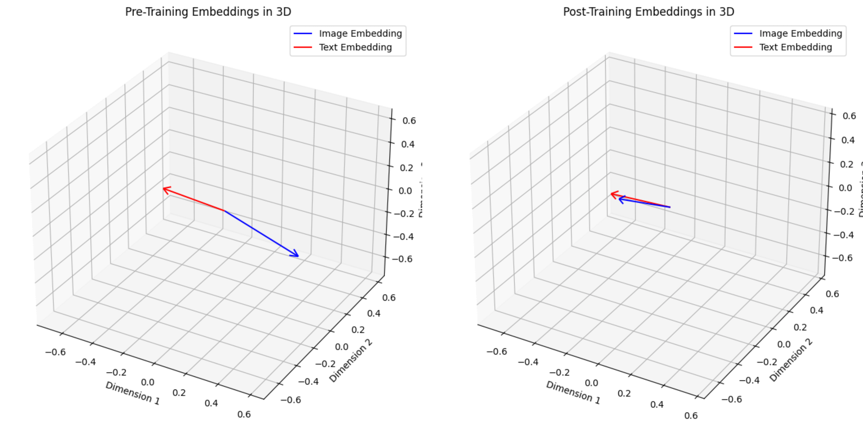
The objective of the model is to represent both images and texts as vectors in a shared embedding space. This idea is central to all vision–language systems.
An image encoder converts an image into a vector zi
A text encoder converts a caption into a vector zt
If zi and zt correspond to the same pair, their cosine similarity should be high
If they belong to different pairs, the similarity should be low
This approach eliminates the need for specific labels. Instead, the model learns a geometric structure in which semantic similarity corresponds to spatial proximity in the embedding space.
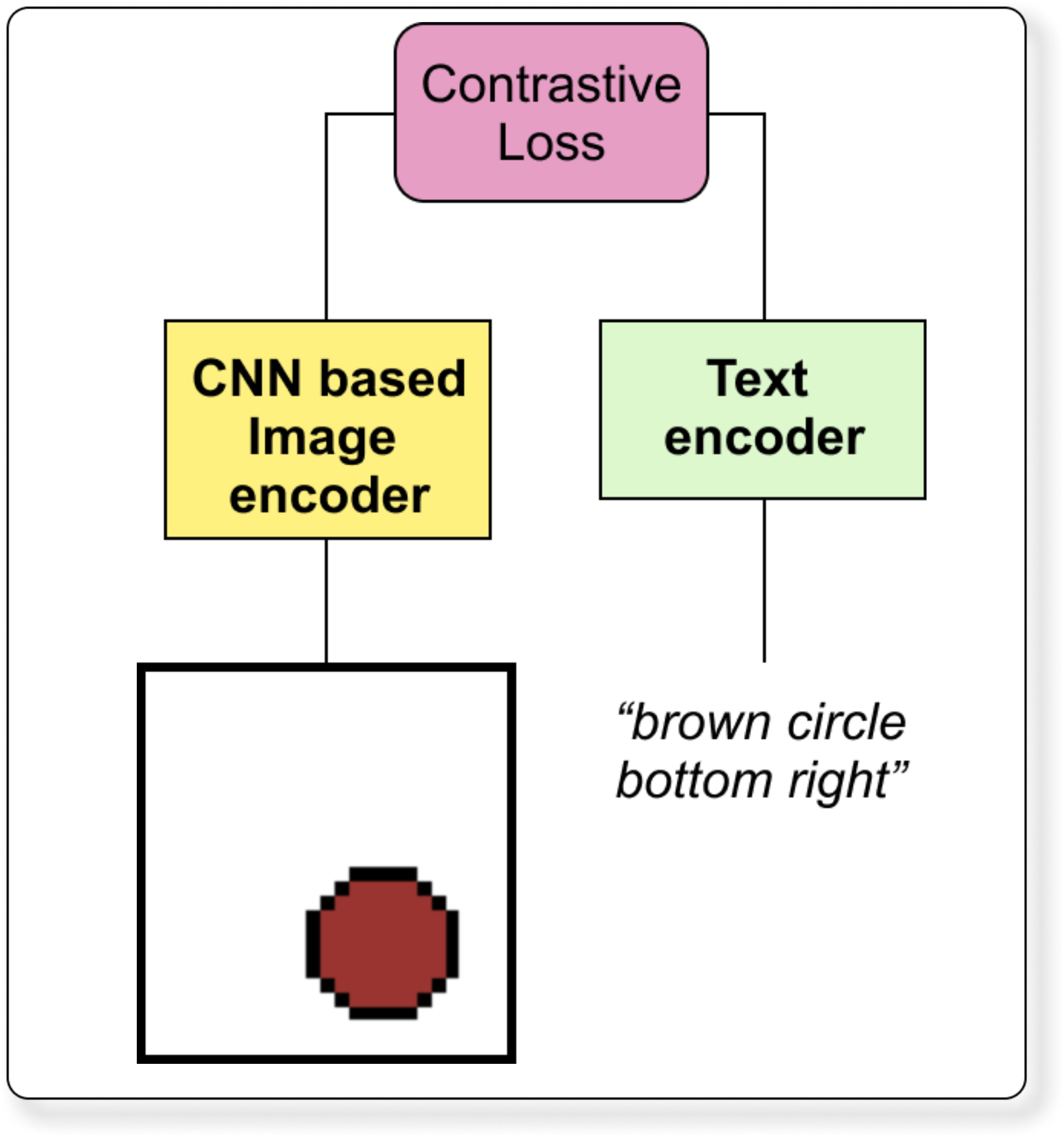
4. Architecture Overview
The nano-VLM follows a dual-encoder architecture similar to CLIP.
4.1 Image Encoder (CNN-based)
A small convolutional neural network is used as the image encoder. The structure gradually reduces spatial dimensions while increasing channel depth.
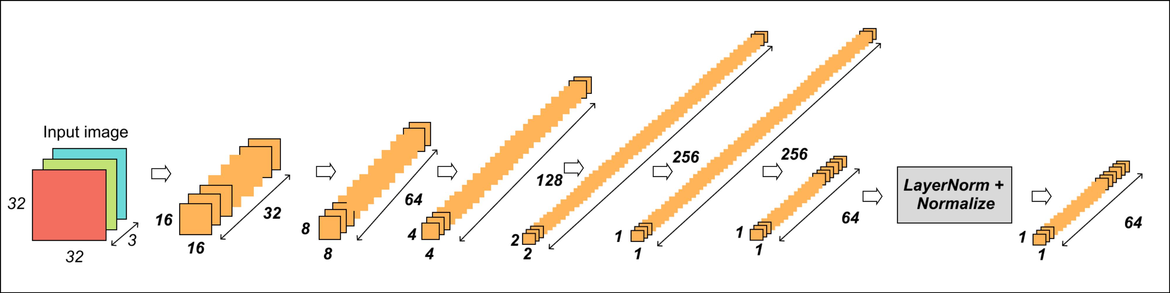
Example architecture:
Input: 32 × 32 × 3 image
→ Conv layer (stride 2) → 16 × 16 × 32
→ Conv layer (stride 2) → 8 × 8 × 64
→ Conv layer (stride 2) → 4 × 4 × 128
→ Conv layer (stride 2) → 2 × 2 × 128
→ Conv layer (stride 2) → 1 × 1 × D  (D = embedding dimension, e.g., 16 or 32)
→ Flatten → LayerNorm → Unit vector (L2 normalization)
The final output is a D-dimensional embedding representing the image.
4.2 Text Encoder
Each caption consists of three words plus a special classification token [CLS].
Example:
CaptionTokenspink circle top[CLS], pink, circle, top
Two variations of the text encoder can be used:
Simple Encoder
Convert tokens to embeddings
Compute the mean of token embeddings
Project to embedding dimension
LayerNorm and L2 normalization
Self-Attention Based Encoder (optional)
Token embeddings + positional embeddings
Multi-head self-attention
Output of the
[CLS]token is taken as final representation
The simple encoder is sufficient for the dataset and is faster to train.
5. Contrastive Loss (CLIP-style)
To train the model, contrastive learning is employed. The training batch contains N images and N corresponding captions.
For each image embedding zi, compute similarity with all caption embeddings in the batch
The highest similarity should be with its paired caption embedding zt
For all other captions in the batch, similarity should be low
This is done twice:
Image-to-Text Loss – image as anchor, all captions as candidates
Text-to-Image Loss – caption as anchor, all images as candidates
The final loss is the average of both. This encourages symmetric alignment.
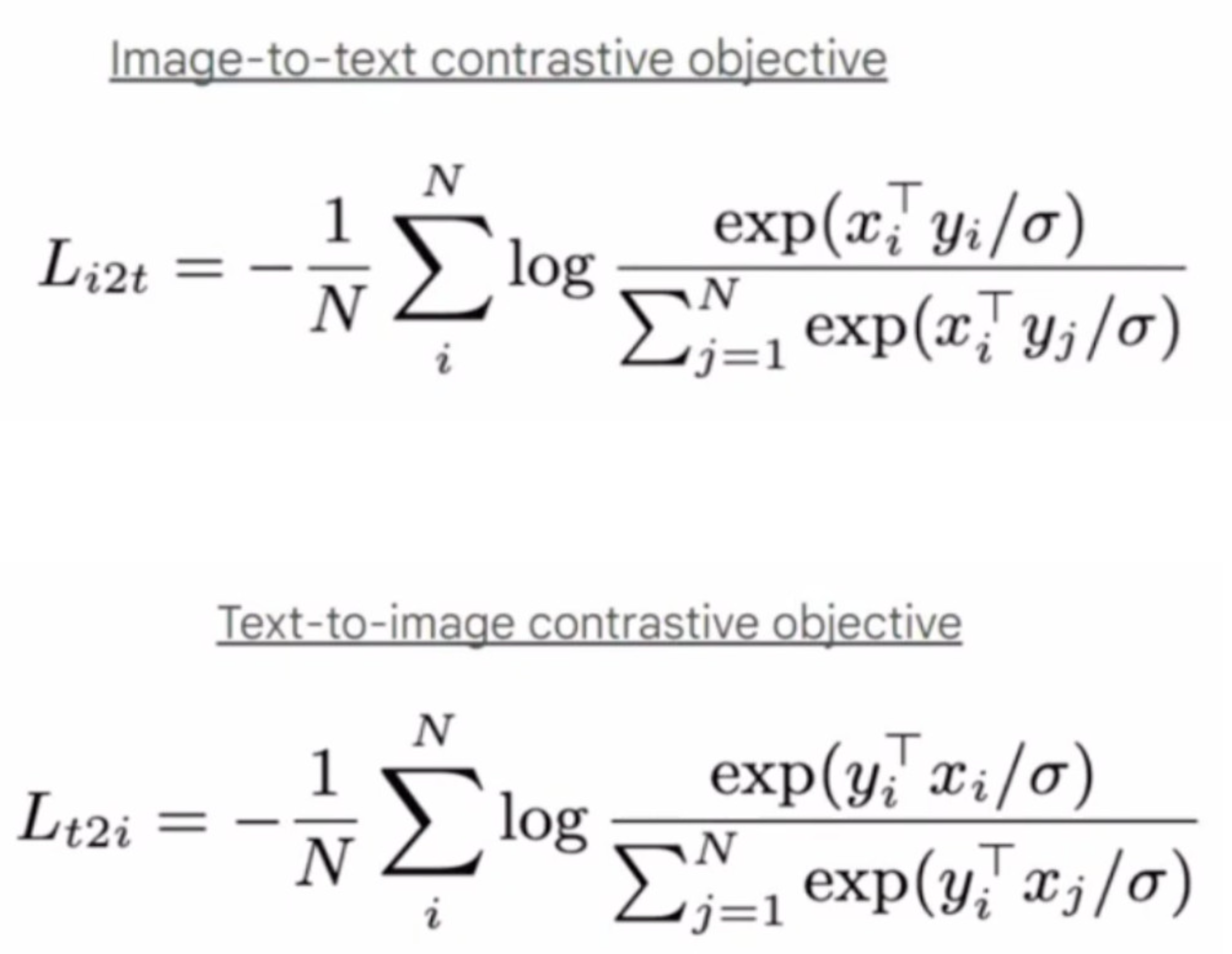
A temperature parameter τ (typically between 0.05 and 0.1) scales the similarity values before applying softmax, controlling how sharp or smooth the probability distribution becomes.
6. Training Pipeline
6.1 Data Splitting
The 243 pairs are divided into:
80 percent for training
20 percent for validation
6.2 Training Loop
For each batch:
Generate image embeddings using the image encoder
Generate caption embeddings using the text encoder
Compute similarity matrix between every image and every caption in the batch
Calculate contrastive loss (image-to-text + text-to-image)
Backpropagate and update encoder parameters
Optimization uses Adam with a fixed learning rate.
7. What the Model Learns
Even though the dataset is extremely small, the model learns meaningful relationships. It begins to understand that:
Changing the position in the caption should change the embedding
Colours and shapes influence the representation distinctly
An incorrect caption such as “yellow triangle bottom-left” should not align with an image of a “green circle top-right”
Validation shows whether the model correctly retrieves images or captions for unseen samples.
8. Importance of This Exercise
Most implementations of VLMs rely on large-scale datasets and pre-trained weights. However, understanding the principles behind these systems requires building them from the ground up.
This nano-VLM demonstrates:
How multimodal datasets can be constructed from basic elements
How dual encoders convert vision and language into a shared embedding space
How contrastive learning aligns the two modalities
How retrieval works without explicit classification
Despite its simplicity, the model captures the full reasoning pipeline used in large-scale systems.
9. Extensions and Future Work
Several meaningful extensions can follow:
Replacing the CNN with a vision transformer
Using transformer-based text encoder with positional embeddings and self-attention
Increasing dataset complexity with multiple objects per image
Applying the model to real-world datasets such as MS COCO
Adding generation capabilities to convert image embedding back into text
Conclusion
Building a nano-scale Vision–Language Model from scratch provides a clear and complete understanding of how multimodal learning systems operate. The model constructs a shared embedding space, learns image–text alignment using contrastive loss, and performs retrieval tasks efficiently even without large datasets or pre-training.
This exercise forms a foundational step towards understanding larger systems such as CLIP, BLIP, Flamingo and GPT-4V.
YouTube lecture
Join PRO
– Access to all lecture videos
– Hand-written notes
– Private GitHub repo
– Private Discord
– “Transformers for Vision” book by Team Vizuara (PDF)
– Email support
– Hands-on assignments
– Certificate