Attention Residuals: Teaching transformers to choose which layers matter

How Moonshot AI replaced a decade-old fixed-weight residual connection with learned depth-wise attention, unlocking 25% more compute efficiency in Kimi

This article covers:

• The PreNorm dilution problem: Why standard residual connections cause hidden states to grow uncontrollably with depth, drowning out individual layer contributions

• The depth-time duality: The elegant insight that information dilution across depth is structurally identical to memory loss across a sequence, and can be solved the same way

• Attention Residuals (AttnRes): How replacing fixed accumulation with softmax attention over previous layer outputs gives each layer selective, input-dependent access to earlier representations

• Block AttnRes: The practical variant that partitions layers into blocks, reducing memory from O(Ld) to O(Nd) while preserving most gains

• Quantifying the gains: Scaling law experiments showing a 1.25x compute advantage, with benchmark improvements up to +7.5 points on GPQA-Diamond

This article assumes familiarity with transformers, self-attention, and residual connections. If you have read about how standard transformer blocks work, including the alternation of attention and feed-forward sublayers connected by residual streams, you have all the background you need.

Let’s begin with a roadmap of what we will cover, as shown in figure 1.

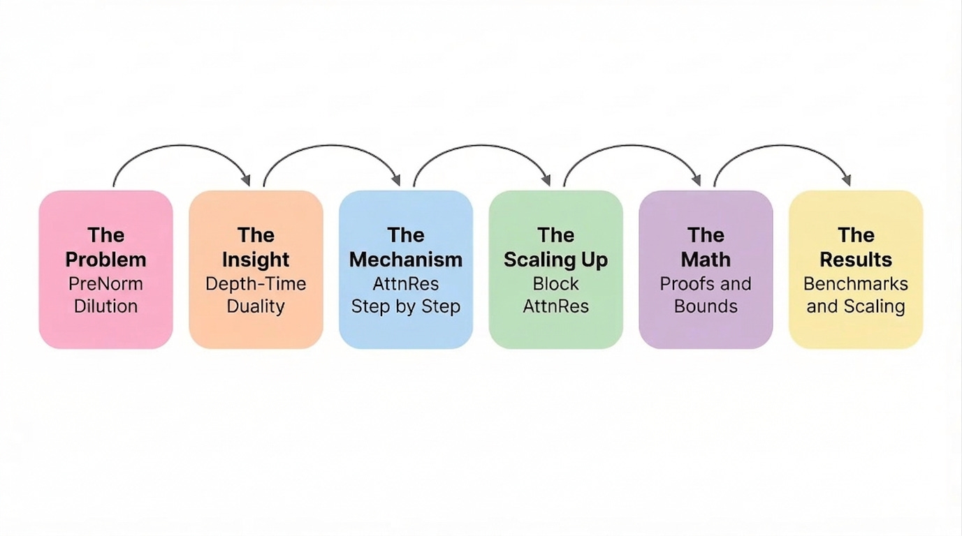
As shown in figure 1, we will progress through six stages. We start by understanding a hidden problem inside every modern LLM, build the conceptual insight that makes the fix possible, walk through the mechanism in detail, scale it to real-world models, prove it works mathematically, and finally measure the gains.

To understand why Attention Residuals matter, we first need to confront a hidden problem lurking inside every modern LLM.

---

The hidden flaw in residual connections

Residual connections are one of the most important innovations in deep learning. Introduced by He et al. in 2016, they allow gradients to flow through deep networks by providing shortcut paths around each layer. Every modern LLM, from GPT to LLaMA to DeepSeek, relies on them.

Yet these connections have a fundamental design limitation that has gone largely unaddressed for a decade. Every layer output is added to the running hidden state with a fixed weight of 1.0, creating an ever-growing signal that progressively drowns out individual layer contributions. This is the PreNorm dilution problem, and it wastes model capacity while limiting the effective utilization of depth.

The residual stream

Let’s examine how residual connections work in a standard PreNorm transformer, as illustrated in figure 2.

Figure 2. The residual stream in a standard transformer. Each layer adds its output to the running sum with a fixed weight of 1.0, creating a single, ever-growing hidden state.

As shown in figure 2, each transformer layer receives the current hidden state, applies RMSNorm, processes it through attention and a feed-forward network, and then adds the result back to the running sum. The formula at each layer is straightforward:

\(h_l = h_{l-1} + f_l(\text{RMSNorm}(h_{l-1}))\)

The key observation is that every layer contributes its output with the same fixed weight of 1.0. There is no mechanism for one layer to contribute more or less than any other. The running sum, often called the “residual stream,” simply accumulates all outputs equally.

For our running example, we use four tokens, “The”, “cat”, “sat”, “down”, each with an 8-dimensional embedding. The input matrix X has shape (4, 8). We trace these tokens through 6 layers.

The magnitude growth problem

Since every layer adds its output with weight 1.0, the hidden state norm grows linearly with depth. This is not a minor bookkeeping detail. It is a fundamental property that shapes how the entire model behaves.

The hidden state at the final layer is literally the sum of all previous outputs:

\(h_L = x + f_1(\text{RMSNorm}(h_0)) + f_2(\text{RMSNorm}(h_1)) + \ldots + f_L(\text{RMSNorm}(h_{L-1}))\)

Let’s see this growth in action with our running example, as shown in figure 3.

Figure 3. Hidden state magnitude growth across depth in a standard PreNorm transformer. The orange line shows the standard residual norm growing linearly with the number of layers, while the gray bars show each individual layer’s fractional contribution shrinking toward zero. The blue line shows AttnRes norm for comparison, staying bounded near 1.0.

As shown in figure 3, the standard residual norm (orange line) grows steadily from 1.0 at the embedding layer to over 5.0 by layer 12. Meanwhile, the layer contribution fraction (gray bars) shrinks from 1.0 at layer 0 to less than 0.1 by layer 12. The RMSNorm before each sublayer normalizes the input, but the accumulated output keeps growing unchecked.

In a 50-layer model, the hidden state is the sum of approximately 50 vectors. Each layer’s contribution represents roughly 2% of the total signal. This is the PreNorm dilution problem.

The signal dilution effect

The consequence of this magnitude growth is that each layer’s voice gets progressively quieter relative to the total signal. Let’s visualize what the final hidden state actually looks like, as shown in figure 4.

Figure 4. The contribution of each layer as a fraction of the total hidden state, shown for a 6-layer model. Layer 1’s output, which might encode crucial low-level features, represents only 1/6 of the final hidden state. In a 50-layer model, each layer is only 2% of the total.

As illustrated in figure 4, the final hidden state h_6 is the sum of 7 components: the token embedding x plus 6 layer outputs f_1 through f_6. Each contributes roughly 14% of the total signal. This means that layer 1, which might encode crucial low-level syntactic features, has the same influence as layer 6, which handles high-level reasoning. There is no selectivity.

This lack of selectivity creates a deeper problem. Both the attention sublayer and the FFN sublayer within each block receive the same blended signal, even though they may benefit from very different mixtures of earlier information.

Evidence of wasted capacity

The dilution problem is not just theoretical. Research has demonstrated that entire layers can be removed from deep LLMs with minimal performance impact, as shown in figure 5.

Figure 5. The redundancy problem. Research has shown that entire layers can be removed from deep LLMs with minimal performance impact, suggesting that uniform accumulation wastes model capacity.

As shown in figure 5, removing 3 middle layers from a 12-layer model results in only a 3% performance drop. This suggests that the uniform accumulation of residual connections makes many intermediate layers effectively redundant. The model cannot efficiently utilize depth because each additional layer has diminishing marginal impact on the blended hidden state.

Now that we see the problem clearly, a natural question arises: can we fix this by applying the same trick that transformers already use to solve a structurally identical problem?

---

The depth-time duality

The conceptual breakthrough behind Attention Residuals comes from a simple but profound observation: the problem of information dilution across network depth is structurally identical to the problem of memory loss across a sequence of tokens. And we already know how to solve the sequence version.

The sequence analogy

Before transformers, recurrent neural networks processed sequences by passing a hidden state from one time step to the next. Early tokens were progressively forgotten as the sequence grew, because each new token blended into the same fixed-size hidden state. This “forgetting” problem limited how far back an RNN could effectively look.

The transformer’s self-attention mechanism solved this elegantly, as shown in figure 6.

Figure 6. The memory loss problem in sequences. Top: Without attention (RNN), early tokens progressively fade as the sequence grows, and the hidden state contains mostly recent information. Bottom: With attention (Transformer), any position can selectively access any previous position with learned, content-dependent weights, preventing the forgetting problem.

As illustrated in figure 6, the transformer replaced the sequential blending of an RNN with selective retrieval via attention. Instead of each position receiving only the previous position’s output, any position can directly attend to any earlier position. The attention weights are content-dependent, meaning the model learns which earlier positions are most relevant for each new token.

Rotating attention from time to depth

Now here is the key insight. In the depth dimension of a transformer, the same “forgetting” problem occurs. Early layer outputs are progressively diluted as more layers are added, just as early tokens were forgotten in RNNs. The fix is structurally identical: let each layer directly access any previous layer with learned, content-dependent weights.

This is what the authors of Attention Residuals describe as “rotating” the attention mechanism 90 degrees, as shown in figure 7.

Figure 7. The depth-time duality. Left: standard self-attention operates horizontally across sequence positions, letting each token attend to previous tokens using softmax-weighted combinations. Right: AttnRes operates vertically across network depth, letting each layer attend to previous layers using the same mathematical structure. The formula h = sum(alpha_i * v_i) is identical in both cases.

As shown in figure 7, both mechanisms compute h = sum(alpha_i * v_i), where the alpha weights are computed via softmax over learned scores. The only difference is the dimension: standard attention operates across sequence positions (horizontal), while AttnRes operates across network depth (vertical).

Let’s visualize this rotation more concretely, as illustrated in figure 8.

Figure 8. Rotating attention 90 degrees. Left: a standard self-attention matrix with token positions on the axes, attending across the sequence (horizontal). Right: an AttnRes attention pattern with layer depths on the axes, attending across depth (vertical). The same causal masking structure applies: each position/layer can only attend to those that came before it.

As shown in figure 8, the standard self-attention matrix (left) has tokens on both axes, with the causal mask ensuring each token only attends to previous tokens. The AttnRes pattern (right) has layers on both axes, with each layer attending only to previous layers. The mathematical structure is the same, just applied to a different dimension.

This is a profound reframing. The residual stream has always been performing a kind of “attention” over depth, but the crudest possible kind: every layer gets weight 1.0 regardless of content. AttnRes upgrades this to full softmax attention with learned, input-dependent weights.

With this duality in mind, let’s see exactly how Attention Residuals work, step by step.

---

The mechanics of Attention Residuals: a hands-on walkthrough

We now have the intuition: replace fixed-weight residual accumulation with softmax attention over previous layer outputs. Let’s build the mechanism piece by piece, starting with a review of what standard residuals compute and ending with the full AttnRes forward pass.

Standard residuals in action

Let’s first trace through our running example with standard residual connections to see the problem concretely. The side-by-side comparison in figure 9 frames what we are about to build.

Figure 9. Standard residual connections vs Attention Residuals. Left: each layer blindly adds its output to the accumulated sum with fixed weight 1.0, and the magnitude grows as O(L). Right: each layer uses a learned pseudo-query vector w_l to selectively weight previous layer outputs via softmax attention, keeping magnitudes bounded.

As illustrated in figure 9, the standard approach (left) produces a hidden state h_4 with growing magnitude because all four layer outputs are summed with equal weight. The AttnRes approach (right) produces a bounded h_4 because the softmax weights, computed via pseudo-query vectors w_1 through w_4, always sum to 1.

Now let’s walk through the standard computation layer by layer, as shown in figure 10.

Figure 10. Standard residual computation for our running example. Four tokens flow through 6 layers, with each layer’s output added with weight 1.0. The hidden state vectors grow progressively larger at each layer, from norm 1.0 at the embedding to norm 3.2 at layer 6. The bar chart on the right confirms the linear O(L) growth.

As shown in figure 10, our tokens start with embedding norm 1.0. After layer 1, the hidden state has norm 1.4 (the sum of the embedding and layer 1’s output). By layer 3, the norm has grown to 2.3. By layer 6, it reaches 3.2. Each layer contributes roughly 0.4 to the total norm, creating steady linear growth.

We can verify this growth pattern across all four of our tokens, as shown in figure 11.

Figure 11. Hidden state magnitudes for our 4 tokens across 6 layers with standard residuals. All four tokens (”The”, “cat”, “sat”, “down”) show monotonically increasing norms, confirming the O(L) growth problem in our running example. The curves are tightly clustered, growing from 1.0 to approximately 3.4-3.6.

As illustrated in figure 11, all four tokens exhibit the same monotonic growth pattern. The norms rise from 1.0 at the embedding layer to between 3.4 and 3.6 by layer 6. This confirms that the dilution problem is universal across all tokens, not specific to any particular input.

The pseudo-query vector

The first new concept in AttnRes is the pseudo-query vector. Each layer l has a learned parameter vector w_l of the same dimension as the hidden state (in our example, d = 8). This vector encodes the question: “which previous layers are most relevant for my computation?”

Let’s examine this concept in detail, as illustrated in figure 12.

Figure 12. The pseudo-query vector. Each layer l has a learned vector w_l of shape (8,) that acts as a “question” asking which previous layers matter most. The pseudo-query computes dot products with RMSNorm-normalized representations from previous layers, producing scores that pass through softmax to yield attention weights. The scores in this example are 0.2, 0.8, 1.5, 0.6 for layers 0-3, producing weights alpha_0=0.05, alpha_1=0.20, alpha_2=0.55, alpha_3=0.20.

As shown in figure 12, the pseudo-query w_l is a fixed learned parameter, not derived from the input like a standard attention query. However, the attention weights are still input-dependent because the “keys” come from previous layer outputs (v_i), which depend on the input tokens. Different inputs produce different keys, which produce different dot products with the same pseudo-query, which produce different attention weights.

What is a pseudo-query? A pseudo-query is a learned parameter vector that functions like a query in standard attention, but instead of being derived from the input, it is a fixed vector that each layer learns during training. It asks the same “question” for every input, but gets different “answers” because the keys (previous layer outputs) vary with the input.

Computing attention weights over depth

Now let’s see the full computation at a single layer. At layer 4, we have four previous outputs to attend over: v_0 (embeddings), v_1 (layer 1 output), v_2 (layer 2 output), and v_3 (layer 3 output). The detailed computation is shown in figure 13.

Figure 13. AttnRes computation at layer 4 in detail. The pseudo-query w_4 computes dot products with RMSNorm-normalized representations from layers 0 through 3, producing logits [0.2, 0.8, 1.5, 0.6]. After softmax, the weights are alpha_0=0.08, alpha_1=0.15, alpha_2=0.55, alpha_3=0.22. The output h_4 = 0.08*v_0 + 0.15*v_1 + 0.55*v_2 + 0.22*v_3 is bounded because the weights form a convex combination.

As shown in figure 13, the computation proceeds in four steps:

1. Normalize: Each previous output v_i is passed through RMSNorm to produce a key k_i

2. Score: The pseudo-query w_4 is dotted with each key to produce logits [0.2, 0.8, 1.5, 0.6]

3. Softmax: The logits are converted to attention weights that sum to 1: [0.08, 0.15, 0.55, 0.22]

4. Aggregate: The output is the weighted sum: h_4 = 0.08v_0 + 0.15v_1 + 0.55v_2 + 0.22v_3

The formal equation for the attention weights is:

\(\alpha_{i \rightarrow l} = \text{softmax}_i(w_l^T \cdot \text{RMSNorm}(k_i)) = \frac{\exp(w_l^T \cdot \text{RMSNorm}(k_i))}{\sum_{j=0}^{l-1} \exp(w_l^T \cdot \text{RMSNorm}(k_j))}\)

Let’s zoom into the attention weight computation itself, as shown in figure 14.

Figure 14. Attention weight computation for layer 4. The pseudo-query w_4 of shape (8,) is dotted with the key matrix K of shape (4, 8) containing the RMSNorm-normalized outputs from layers 0-3. The dot products produce logits of shape (4,): [0.2, 0.8, 1.5, 0.6]. After softmax, the resulting weights are alpha_0=0.08, alpha_1=0.15, alpha_2=0.55, alpha_3=0.22. The bar chart shows that layer 4 draws 55% of its input from layer 2’s output, making it the dominant source.

As illustrated in figure 14, layer 4 selectively draws 55% of its input from layer 2’s output. Notice how different this is from standard residuals, where all layers contribute equally. The model has learned that layer 2’s representation is the most useful input for layer 4’s computation, and it can focus its attention accordingly.

The full AttnRes forward pass

Now let’s trace the complete forward pass with AttnRes through all 6 layers of our running example, as shown in figure 15.

Figure 15. Full AttnRes computation for our running example. The same 4 tokens flow through 6 layers, but each layer selectively weights its inputs via softmax attention. At layer 1, alpha_0 = 1.0 (only the embeddings are available). At layer 2, the weights are [0.3, 0.7]. At layer 3, the weights are [0.1, 0.2, 0.7]. The hidden state magnitudes remain bounded throughout: norms stay between 0.95 and 1.1, compared to the 1.0 to 3.2 range with standard residuals.

As shown in figure 15, the hidden state magnitudes stay bounded near 1.0 throughout all 6 layers. This is a dramatic contrast with the standard residual version, where magnitudes grew to 3.2. The key difference is visible in the bar chart on the right: instead of linearly increasing bars, we see roughly uniform bars that stay below the dashed line marking the standard residual growth.

Let’s confirm this with a direct comparison of the magnitude curves, as shown in figure 16.

Figure 16. Hidden state magnitudes comparison. The orange line (Standard Transformer) grows linearly from 1.0 to 3.45 over 6 layers. The blue line (Attention Residual) stays flat near 1.0, oscillating between 0.95 and 1.05. This bounded behavior is a direct consequence of the convex combination property: since softmax weights sum to 1, the output magnitude can never exceed the largest input magnitude.

As illustrated in figure 16, the difference is stark. The standard residual norm (orange) grows from 1.0 to 3.45 over just 6 layers. The AttnRes norm (blue) stays essentially flat near 1.0. This is the mathematical magic of Attention Residuals: by replacing fixed-weight accumulation with a softmax-weighted combination, the hidden state magnitude is automatically bounded.

Input-dependent layer selection

The final piece of the puzzle is that different tokens produce different attention weight distributions. This is what makes AttnRes strictly more expressive than fixed-weight approaches like DenseFormer. Let’s see this in action, as shown in figure 17.

Figure 17. Input-dependent attention weights. The same pseudo-query w_4 produces different weight distributions for different tokens. Token “The” (a function word) attends mostly to the embedding layer (alpha_0 = 0.60). Token “cat” (a content word) focuses on intermediate layers (alpha_2 = 0.55). Token “down” (context-dependent) attends most to recent layers (alpha_3 = 0.40). This input-dependence is what makes AttnRes strictly more expressive than DenseFormer.

As shown in figure 17, the same pseudo-query w_4 produces three very different attention patterns depending on the token:

• Token “The”: A function word that attends mostly to the embedding layer (alpha_0 = 0.60). Function words carry relatively stable syntactic information that does not change much across layers.

• Token “cat”: A content word that focuses on intermediate layers (alpha_2 = 0.55). Content words benefit from the semantic processing performed by middle layers.

• Token “down”: A context-dependent word that attends most to recent layers (alpha_3 = 0.40). Its meaning depends heavily on the context built up by previous layers.

This is the key advantage over fixed-weight approaches. DenseFormer uses the same weights for every token; AttnRes adapts its layer selection to each token individually.

We now have the full AttnRes mechanism, but there is a practical challenge: storing all L layer outputs requires O(Ld) memory. For massive models with tens of billions of parameters, we need a more efficient approach.

---

Block AttnRes: scaling to real-world models

Full AttnRes is elegant but expensive. At layer l, we need to store all l-1 previous outputs, each of dimension d. For a 48-layer model with d = 8192, this represents significant memory overhead. In pipeline-parallel training, where different layers live on different GPUs, the situation is even more challenging.

The solution is Block AttnRes, which partitions layers into blocks and applies attention only at block boundaries.

The memory challenge

Let’s first understand the architecture at a high level, as shown in figure 18.

Figure 18. Block AttnRes architecture. Layers are partitioned into blocks (shown here with 4 blocks of 6 layers each for a 24-layer model). Within each block, standard residual connections accumulate outputs with weight 1.0. At block boundaries, attention-based aggregation selectively combines all previous block representations plus the original token embedding. Memory is O(Nd) instead of O(Ld).

As shown in figure 18, Block AttnRes uses standard residuals within blocks (the familiar h_l = h_{l-1} + f_l pattern) but applies attention-based aggregation at the boundaries between blocks. The token embeddings x are always available as one of the attention sources, providing a direct path from input to any block.

The memory savings are substantial, as illustrated in figure 19.

Figure 19. Memory comparison. Full AttnRes stores all 48 layer outputs, requiring O(L*d) = O(48*d) memory. Block AttnRes stores only 8 block-level representations plus the embeddings, requiring O(N*d) = O(8*d) memory. For a 48-layer model with 8 blocks, this is a 6x reduction in stored representations.

As illustrated in figure 19, full AttnRes requires storing 48 separate representations for a 48-layer model. Block AttnRes with N = 8 blocks stores only 9 representations (8 block outputs plus the token embeddings), a 6x reduction. The authors found that 8 blocks is the optimal trade-off between performance and overhead.

How Block AttnRes works

Let’s walk through Block AttnRes with our running example: 6 layers partitioned into 2 blocks of 3 layers each. The step-by-step computation is shown in figure 20.

Figure 20. Block AttnRes step-by-step for our running example with L=6 layers and N=2 blocks. Block 1 (Layers 1-3) uses standard residuals internally with weight 1.0. At the block boundary, attention aggregates the token embeddings x and Block 1’s output B_1 with weights alpha_x = 0.35 and alpha_B1 = 0.65, producing h_boundary. Block 2 (Layers 4-6) then proceeds with standard residuals using h_boundary as input.

As shown in figure 20, the computation proceeds in three phases:

1. Block 1 (Layers 1-3): Standard residual connections. Each layer adds its output to the running sum. The block output B_1 = h_3 has a growing magnitude, just like in a standard transformer.

2. Block boundary: The attention mechanism computes weights over the token embeddings x and block 1’s output B_1. In this example, the weights are alpha_x = 0.35 and alpha_B1 = 0.65, producing h_boundary = 0.35x + 0.65B_1. This “resets” the magnitude by forming a convex combination.

3. Block 2 (Layers 4-6): Standard residual connections resume, using h_boundary as the starting point.

Notice the critical design insight: within blocks, O(L) growth is allowed to occur. But at block boundaries, the attention-based aggregation “resets” the magnitude back to a bounded value. This means the maximum growth within any single block is limited to O(L/N), which is much smaller than O(L).

Now let’s examine the block boundary computation in more detail, as shown in figure 21.

Figure 21. Attention computation at a block boundary. In Stage 1 (Stack), the token embeddings, previous block outputs, and current partial sum are gathered. In Stage 2 (Normalize), all sources are normalized with RMSNorm. In Stage 3 (Score), the learned projection weight (pseudo-query) computes attention logits via einsum, then softmax produces weights. In Stage 4 (Aggregate), the weighted sum produces the aggregated block input for the next block.

As illustrated in figure 21, the block boundary attention follows four stages:

1. Stack: Gather the token embeddings, all previous block outputs, and the current block’s partial sum into a tensor V of shape (N_prev+1, batch, seq, d)

2. Normalize: Apply RMSNorm to stabilize the attention computation

3. Score: Use the learned projection weight (the pseudo-query) to compute logits via einsum, then apply softmax to get weights

4. Aggregate: Compute the weighted sum to produce the input for the next block

Pipeline parallelism and system design

In large-scale training, models are split across multiple GPUs using pipeline parallelism. Each GPU holds a subset of layers, typically corresponding to one or two blocks. The challenge is that block boundary attention needs representations from blocks on other GPUs.

The solution is cache-based point-to-point communication, as shown in figure 22.

Figure 22. Block AttnRes in pipeline-parallel training. Four GPUs each hold 2 blocks. Each GPU caches its block representations and sends them to the next GPU via point-to-point communication. GPU 0 caches [x, B_1, B_2] and sends [B_1, B_2] to GPU 1. GPU 1 adds its own block outputs and forwards [B_1..B_4] to GPU 2, and so on. Each GPU runs a two-phase computation: Phase 1 computes standard attention within the current block, Phase 2 applies cross-block attention using cached representations.

As shown in figure 22, each GPU stage maintains a cache of all block representations computed so far. When a block boundary is reached, the cached representations from previous stages are available for the attention computation. The two-phase strategy ensures efficient execution:

• Phase 1: Compute the standard attention and FFN operations within the current block

• Phase 2: Apply cross-block attention using the cached block representations

During inference, online softmax is used to amortize the computation cost, keeping the overhead minimal.

Having built the complete mechanism, both the idealized full version and the practical block variant, let’s formalize the mathematics and prove why AttnRes solves the dilution problem.

---

The mathematics of Attention Residuals

We have built intuition for why AttnRes works. Now let’s prove it. The mathematics reveals three key properties: bounded hidden states, improved gradient flow, and a beautiful connection between standard residuals and linear attention.

Bounding the hidden state

The most important mathematical property of AttnRes is that it produces a convex combination of previous outputs. Since softmax weights sum to 1, the output magnitude is automatically bounded, as shown in figure 23.

Figure 23. The convex combination bound. Top: Standard residuals compute h_L = v_0 + v_1 + v_2 + ... + v_L, and the magnitude can grow as O(L). AttnRes computes h_L = alpha_0*v_0 + alpha_1*v_1 + ... + alpha_L*v_L where the alphas sum to 1, and the magnitude satisfies the bound: norm of h_L is at most the maximum norm of any v_i. Bottom: the geometric intuition shows that the AttnRes output always lies within the convex hull of the input vectors, while the standard residual output can escape far beyond this region.

As illustrated in figure 23, the bound is elegantly simple:

Standard residuals:

\(\|h_L\| = \|\sum_{i=0}^{L} v_i\| \text{ can grow as } O(L)\)

AttnRes:

\(\|h_L\| = \|\sum_{i=0}^{L} \alpha_i v_i\| \leq \max_i \|v_i\| \text{ (bounded)}\)

This follows directly from the triangle inequality and the fact that the alpha weights are non-negative and sum to 1. The output is a weighted average of the input vectors, and a weighted average can never have a larger magnitude than the largest input. This single property eliminates the entire PreNorm dilution problem, regardless of how many layers the model has.

Gradient flow and training dynamics

The second mathematical advantage concerns gradient flow during training. In standard residuals, gradients must propagate backward through a chain of multiplicative terms. In AttnRes, each layer receives a direct gradient signal.

Let’s compare the two gradient flow patterns. The standard residual gradient flow is shown in figure 24.

Figure 24. Gradient flow in standard residuals. The gradient from the loss must propagate backward through a chain of (L-l) multiplicative terms: dL/dh_l = dL/dh_L * product of (I + df_k/dh). While the identity shortcut helps, gradients still concentrate in shallow layers (near the loss) and attenuate for deeper layers (far from the loss). The bar chart on the right shows gradient norms heavily concentrated in recent layers.

As shown in figure 24, the standard gradient formula involves a product of (L-l) Jacobian terms. While the identity component of each term helps prevent complete vanishing, the gradients still tend to concentrate in the layers closest to the loss, leaving early layers with weaker gradient signals.

Now let’s examine the AttnRes gradient flow, as shown in figure 25.

Figure 25. Gradient flow in AttnRes. Each layer receives a direct gradient signal weighted by its attention weight alpha. Layers that contribute more to the output (higher alpha) get proportionally stronger gradient signals. This creates a self-reinforcing learning dynamic: useful layers get trained more effectively. The bar chart shows gradient norms distributed much more uniformly across depth.

As illustrated in figure 25, AttnRes provides each layer with a direct gradient path:

\(\frac{\partial \mathcal{L}}{\partial v_l} = \sum_{k=l+1}^{L} \alpha_{l \rightarrow k} \cdot \frac{\partial \mathcal{L}}{\partial h_k} + \text{(attention weight gradient terms)}\)

Every layer receives a gradient signal weighted by its attention weight alpha. Layers that contribute more to the output get proportionally stronger gradients, creating a self-reinforcing learning dynamic: useful layers train faster, become even more useful, and receive even stronger gradients.

We can verify this improved gradient distribution quantitatively, as shown in figure 26.

Figure 26. Gradient norm distribution across layers. The orange line (Standard) shows gradients growing from 0.15 at layer 1 to 1.0 at layer 8, with early layers receiving much weaker gradient signals. The blue line (AttnRes) shows stable gradient norms between 0.82 and 0.97 across all layers, enabling effective training at every depth.

As shown in figure 26, the standard transformer (orange) shows a severe gradient imbalance: layer 1 receives a gradient norm of only 0.15, while layer 8 receives 1.0. The AttnRes model (blue) maintains gradient norms between 0.82 and 0.97 across all layers. This near-uniform distribution means every layer can train effectively, regardless of its position in the network.

Standard residuals as low-rank linear attention

The paper establishes a beautiful theoretical result: standard residual connections are equivalent to low-rank linear attention over depth. This reframing reveals that the residual stream has always been performing attention over depth, just a very limited form of it. The comparison is shown in figure 27.

Figure 27. Standard residuals as low-rank linear attention. Left: standard residuals compute h_L = sum(1 * v_i) with fixed weight 1.0 for all layers, providing no selectivity. Center: this is equivalent to linear attention with constant weights w_i = 1. Right: AttnRes generalizes this to full-rank softmax attention with input-dependent, learned weights, providing full selectivity. The progression from left to right represents increasing expressiveness.

As illustrated in figure 27, the standard residual sum is mathematically identical to linear attention with constant weights over depth. AttnRes simply upgrades this to full softmax attention, providing strictly more expressive depth-wise information routing. The residual stream has always been doing a form of attention over depth; AttnRes just makes it a much better form.

The math confirms what our intuition suggested: AttnRes fundamentally solves the dilution problem. Now, let’s see how much this matters in practice.

---

Quantifying the gains

Theory is important, but the question practitioners care about is: does it work, and how much does it cost? The Kimi team evaluated Block AttnRes across scaling law experiments, benchmark evaluations, and architecture search, and the results are compelling.

Scaling law experiments

The most informative experiment compares validation loss at different compute budgets. The results are shown in figure 28.

Figure 28. Scaling law curves for standard residuals vs Block AttnRes. Validation loss is plotted against training compute on a log scale. AttnRes (blue) consistently achieves lower loss at every compute budget. The annotation shows that AttnRes matches the standard baseline trained with approximately 25% more compute, meaning a model with AttnRes is equivalent to a 25% larger standard model.

As shown in figure 28, the AttnRes curve (blue) is consistently below the standard curve (orange) at every compute budget from 0.5 to 128 x 10^18 FLOPs. The key result is annotated on the plot: Block AttnRes matches baseline performance trained with 1.25x more compute. This means that adding AttnRes to your model is equivalent to increasing your compute budget by 25%, for free.

Benchmark results

The scaling law result is confirmed by benchmark evaluations on Kimi Linear, a production model with 48B total parameters (3B activated via mixture-of-experts), trained on 1.4 trillion tokens. The results are shown in figure 29.

Figure 29. Benchmark results comparing baseline vs AttnRes on Kimi Linear. The grouped bar chart shows improvements across all 9 benchmarks. The largest gains appear in multi-step reasoning (GPQA-Diamond +7.5 points) and mathematics (Math +3.6 points). Coding tasks also improve significantly (HumanEval +3.1 points). Even knowledge-heavy benchmarks like MMLU and CMMLU show modest but consistent improvements.

As illustrated in figure 29, AttnRes delivers consistent improvements across all 9 benchmarks:

• GPQA-Diamond: +7.5 points (36.9 to 44.4). This is the standout result. GPQA-Diamond tests graduate-level reasoning, and the 7.5-point improvement suggests AttnRes significantly enhances the model’s ability to chain multi-step reasoning.

• Math: +3.6 points (53.5 to 57.1). Mathematical problem-solving requires precise, sequential reasoning across many steps, exactly the kind of task where selective layer access matters most.

• HumanEval: +3.1 points (59.1 to 62.2). Code generation benefits from the improved depth-wise routing, likely because different layers specialize in different aspects of code understanding.

• C-Eval: +2.9 points (79.6 to 82.5). Even on knowledge-focused benchmarks, the improvements are meaningful.

Deeper models, narrower architectures

AttnRes does not just improve performance at a fixed architecture. It fundamentally changes the optimal architecture itself, as shown in figure 30.

Figure 30. Optimal depth-to-width ratio. Left panel: At each depth, AttnRes achieves optimal performance with a narrower model than standard residuals. For example, at 48 layers, the standard optimal width is 4096 while the AttnRes optimal width is 3072. Right panel: At the optimal configuration, AttnRes achieves lower validation loss at every depth, with the advantage growing larger at greater depths. The minimum loss for AttnRes occurs at 64 layers with width 2560, while standard residuals bottom out at 36 layers with width 5120.

As shown in figure 30, standard residuals favor shallower, wider architectures because depth is poorly utilized (due to dilution). AttnRes shifts the optimal point toward deeper, narrower architectures because depth is now effectively utilized through selective attention. This is a fundamental shift in model design philosophy: with AttnRes, you can build deeper models that actually benefit from their depth.

Overhead analysis

The final question is cost. How much overhead does Block AttnRes add? The answer, shown in figure 31, is remarkably little.

Figure 31. Overhead breakdown for Block AttnRes. Left panel (Cost): Training cost increases by only 3.8%, and inference latency increases by only 1.9%. Right panel (Benefits): The gains far outweigh the costs. The compute advantage is 25% (equivalent to 1.25x more training compute), GPQA-Diamond improves by 7.5 points, Math by 3.6 points, and HumanEval by 3.1 points.

As illustrated in figure 31, the overhead is minimal:

• Training cost increase: 3.8%. The additional attention computation at block boundaries adds less than 4% to the total training cost.

• Inference latency increase: 1.9%. Block attention is fast relative to the standard attention within layers.

The 1.25x compute advantage far outweighs the less than 4% overhead. For every dollar you spend on the attention computation, you get 25 cents of equivalent compute back in model quality. The authors confirmed that 8 blocks is the optimal trade-off between performance and overhead.

These improvements did not emerge from a vacuum. Attention Residuals represent the latest step in a decade-long quest to improve how deep networks combine information across depth.

---

The evolution of depth-wise aggregation

To appreciate where AttnRes sits in the landscape, it helps to trace the history of how researchers have approached the problem of combining information across depth.

From ResNet to AttnRes: a ten-year journey

The progression from fixed residual connections to learned depth-wise attention has unfolded over a decade, as shown in figure 32.

Figure 32. The evolution of depth-wise aggregation in deep learning. From ResNet (2016, fixed weight 1.0 addition) through DenseNet (2016, concatenate all outputs), DenseFormer (Feb 2024, learned input-independent scalar weights), ResFormer (Oct 2024, value residual connections from layer 1), DeepCrossAttention (2025, input-dependent cross-layer weights), to AttnRes (2026, full softmax attention over depth via pseudo-queries). The arrow shows increasing expressiveness from fixed and uniform to learned and selective.

As shown in figure 32, each step in this timeline adds more expressiveness to depth-wise information routing:

• ResNet (2016): Fixed weight 1.0. Every layer contributes equally. Zero overhead, but no selectivity.

• DenseNet (2016): Concatenates all previous outputs instead of summing them. Very expressive but memory-intensive. Primarily used in computer vision.

• DenseFormer (Feb 2024): Learns scalar weights per layer pair, but these weights are input-independent. Minimal overhead, but limited expressiveness.

• ResFormer (Oct 2024): Adds residual connections specifically to value vectors from the first layer. Addresses the related but different problem of attention concentration.

• DeepCrossAttention (2025): Uses full input-dependent cross-attention between layers. Claims up to 3x training speedup. Most similar to AttnRes in concept.

• AttnRes (March 2026): Full softmax attention over depth via a single pseudo-query per layer. Less than 2% inference overhead with 1.25x compute advantage.

Comparing the approaches

A detailed comparison of the key methods is shown in figure 33.

Figure 33. Comparison of depth-wise aggregation methods across five dimensions: weights type, input-dependence, overhead, and key property. Standard residuals use fixed weights with 0% overhead but O(L) growth. DenseFormer uses learned scalars that are input-independent. ResFormer targets attention concentration rather than hidden state dilution. DeepCrossAttention is the first fully input-dependent method. AttnRes achieves input-dependent softmax attention with less than 2% inference overhead and bounded magnitudes.

As illustrated in figure 33, AttnRes occupies a unique position in the design space: it provides full input-dependent attention over depth with less than 2% inference overhead. The key distinguishing properties are bounded magnitudes (from the convex combination) and the 1.25x compute advantage (from better depth utilization).

When does AttnRes struggle?

No technique is universally superior, and AttnRes is no exception. Ziming Liu of MIT and Caltech provides a nuanced analysis of when AttnRes excels and when it falls short.

AttnRes excels on structured tasks where skipping intermediate layers is valuable. Natural language has rich hierarchical structure, with different layers specializing in syntax, semantics, and reasoning. The attention mechanism can learn to focus on specific layers without needing to suppress intermediate representations.

However, AttnRes can struggle on pure memorization tasks where uniform blending works fine. If the task requires every layer’s contribution equally, the selective attention provides no advantage and may even hurt by constraining the representation.

There is also a risk of representation collapse: if the attention weights converge to a uniform distribution during training, AttnRes degenerates to averaging all previous hidden states. This uniform bias can limit expressive capacity in certain settings. Natural language’s structured nature likely explains why Kimi’s strong empirical results generalize well across diverse benchmarks.

Having explored the theory, results, and context, let’s look inside a trained model to see what patterns the depth-wise attention actually learns.

---

Inside a trained model

The most illuminating way to understand AttnRes is to examine what the model actually learns. What patterns do the attention weights develop? How do different blocks interact?

What the attention weights learn

The attention weight heatmap from a trained Kimi Linear model reveals striking patterns, as shown in figure 34.

Figure 34. Learned depth-wise attention weight heatmap from the Kimi Linear 48B model. Source blocks on the x-axis, target blocks on the y-axis. Dark blue indicates high attention weight. Three notable patterns emerge: (1) Early blocks attend strongly to the token embeddings (column 0 is dark for rows 1-2). (2) Middle blocks attend primarily to nearby predecessors (the diagonal is prominent for rows 3-5). (3) Deep blocks develop long-range connections back to early layers (rows 7-8 have dark cells in columns 0-1), suggesting they retrieve fundamental features directly.

As shown in figure 34, three distinct patterns emerge from the learned attention weights:

• Early blocks attend to embeddings: Blocks 1 and 2 place strong attention on the token embeddings (source block 0). This makes sense because early processing needs direct access to the raw input features.

• Middle blocks attend to neighbors: Blocks 3 through 5 show a strong diagonal pattern, attending primarily to their immediate predecessors. This suggests a sequential refinement strategy where each block builds on the most recent computation.

• Deep blocks develop long-range connections: Blocks 7 and 8 show renewed attention to early blocks (columns 0-1), even though they also attend to nearby blocks. This is the most intriguing pattern: deep layers “reach back” to retrieve fundamental features that may have been diluted by intermediate processing.

These patterns would be impossible with standard residual connections, where every block receives the same blended signal regardless of what it needs.

Implementation walkthrough

The implementation of Block AttnRes is remarkably concise. The annotated pseudocode is shown in figure 35.

Figure 35. Annotated PyTorch pseudocode for Block AttnRes. The function block_attn_res takes block representations, a partial sum, and a learned projection. Step 1: Stack all sources into tensor V. Step 2: Normalize with RMSNorm. Step 3: Compute logits via einsum between the projection weight and V. Step 4: Apply softmax over the block dimension (dim=0) to get weights that sum to 1. Step 5: Weighted aggregation via einsum to produce the bounded output.

As illustrated in figure 35, the entire Block AttnRes computation fits in five steps:

def block_attn_res(block_reprs, partial_sum, proj):
    # Step 1: Stack all sources
    V = stack(block_reprs + [partial_sum])      # (N+1, batch, seq, d)

    # Step 2: Normalize
    V = RMSNorm(V)

    # Step 3: Compute attention logits
    logits = einsum('d, n b t d -> n b t',
                    proj.weight.squeeze(), V)

    # Step 4: Softmax over block dimension
    weights = logits.softmax(dim=0)

    # Step 5: Weighted aggregation
    output = einsum('n b t, n b t d -> b t d',
                    weights, V)

    return output

The function takes the previous block representations, the current block’s partial sum, and a learned projection (the pseudo-query). The stack, normalize, score, softmax, aggregate pattern is clean and efficient. Adding Block AttnRes to an existing transformer requires modifying only the block boundary logic, making it a true drop-in replacement for standard residual connections.

---

Summary

We have traced the complete story of Attention Residuals, from the problem they solve to the mechanism they use to the gains they deliver. Let’s recap the key takeaways.

• The PreNorm dilution problem: Standard residual connections add all layer outputs with fixed weight 1.0, causing hidden state magnitudes to grow as O(L) with depth. This progressively dilutes each layer’s contribution, making deeper layers less effective and wasting model capacity. In a 50-layer model, each layer represents only 2% of the final hidden state.

• The depth-time duality: Information dilution across network depth is structurally identical to memory loss across a sequence. Just as self-attention solved the sequence problem by enabling selective access to any previous position, AttnRes solves the depth problem by enabling selective access to any previous layer. The mathematical structure is the same, just rotated 90 degrees.

• The AttnRes mechanism: Each layer uses a learned pseudo-query vector to compute softmax attention weights over all previous layer outputs, producing an input-dependent weighted combination. Since softmax weights sum to 1, the resulting hidden state is a bounded convex combination that can never exceed the magnitude of the largest input. This completely eliminates the O(L) growth problem while providing each layer with selective, content-aware access to earlier representations.

• Block AttnRes for scalability: The practical variant partitions layers into approximately 8 blocks, using standard residuals within blocks and attention-based aggregation at block boundaries. This reduces memory from O(Ld) to O(Nd) while recovering most of the full AttnRes gains. Pipeline-parallel training is supported through cache-based point-to-point communication of block representations, with less than 2% inference overhead.

• Quantified improvements: Block AttnRes achieves a 1.25x compute advantage, matching baseline models trained with 25% more resources. On Kimi Linear (48B total, 3B activated, 1.4T tokens), it improved GPQA-Diamond by +7.5 points, Math by +3.6 points, and HumanEval by +3.1 points. The largest gains appear in multi-step reasoning tasks. AttnRes also shifts the optimal architecture toward deeper, narrower models that more effectively utilize their depth.

---

Further reading

• Attention Residuals (arXiv:2603.15031) - The original paper by Chen et al. at Moonshot AI (Kimi team), March 2026. Full mathematical formulation, scaling law experiments, and Kimi Linear integration.

• MoonshotAI/Attention-Residuals on GitHub - Official implementation with PyTorch pseudocode, Block AttnRes details, and benchmark tables.

• When Does Attention Residuals Work? (Ziming Liu) - Critical analysis from MIT/Caltech showing when AttnRes excels (structured tasks) and when it struggles (pure memorization).

• DenseFormer (arXiv:2402.02622) - The predecessor using Depth-Weighted Averaging with input-independent scalar weights. Important comparison point.

• DeepCrossAttention (arXiv:2502.06785) - Google’s learnable input-dependent cross-layer weights, claiming 3x training speedup.

• Value Residual Learning / ResFormer (arXiv:2410.17897) - Residual connections on value vectors to address attention concentration, saving 10-14% parameters.