
An beginners introduction to Swin transformer
Why did Microsoft introduce the idea of "shifted window" attention?


Table of Content
Introduction to Swin Transformer
Limitations of Vision Transformers at High Resolution
Window Based Attention in Swin Transformers
Hierarchical Feature Representation in Swin Transformers
Overview of the Swin Transformer Architecture
Patch Partitioning and Linear Embedding
Patch Merging and Hierarchical Downsampling
Attention Complexity in Swin Transformers
Shifted Windows for Long Range Interaction in Swin Transformer
Relative Position Bias Parameterization in Swin Transformer
Absence of Class Token in Swin Transformer
Output Heads and Task Generalization
Comparison with Convolutional Backbones
Concluding Remarks on Swin Transformer
1.1 Introduction to Swin Transformer
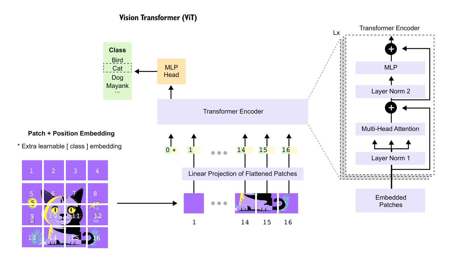
Figure 1.1 Vision Transformer overview.
An input image is divided into fixed size patches, flattened, linearly projected, and combined with positional embeddings to form a sequence of tokens processed by a standard transformer encoder.
The final image representation is obtained from a dedicated class token and passed to an MLP head for prediction.
Transformer based models have reshaped computer vision by reformulating images as sequences of tokens. An input image, represented by its height, width, and color channels, is first partitioned into fixed size spatial patches. Each patch is flattened into a vector and treated as a token, enabling the direct application of self attention mechanisms originally developed for language modeling. This formulation allows the model to capture long range dependencies across the image, but it also exposes a key limitation. As image resolution increases, the number of patches grows proportionally, and the computational and memory cost of self attention scales quadratically with the number of tokens.
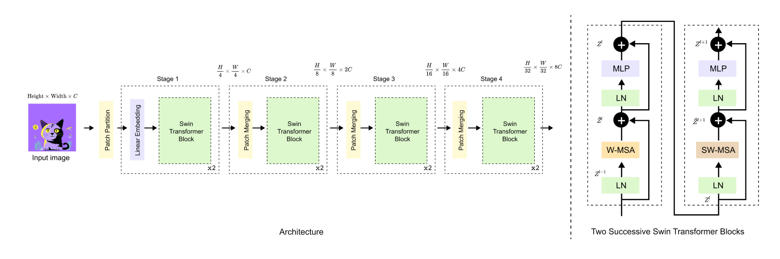
Figure 1.2 Swin Transformer architecture.
The input image is hierarchically processed through multiple stages, where patch partitioning and merging progressively reduce spatial resolution while increasing feature dimensionality.
Each stage is composed of successive Swin Transformer blocks that alternate between window based and shifted window self attention, enabling efficient local computation with cross window information exchange.
The Swin Transformer, short for shifted window transformer, was proposed to overcome this scalability challenge while retaining the expressive power of transformer architectures. Instead of computing attention globally over all image patches, Swin Transformer restricts self attention to local windows and introduces a systematic window shifting strategy across layers. This design enables efficient computation at high resolutions while still allowing information exchange beyond local neighborhoods. As a result, Swin Transformer serves as a strong and scalable backbone for a wide range of visual tasks. In the next section, we will place this architecture in context by contrasting it with earlier vision transformer designs.
1.2 Limitations of Vision Transformers at High Resolution
Vision Transformers model images as a sequence of patch tokens and apply global self attention over all tokens. While this design enables strong long range interactions, it introduces a fundamental computational bottleneck. For an image of height H and width W, divided into patches of size P, the total number of tokens is
Self attention computes interactions between all query key pairs, resulting in an attention complexity that scales as O(N²). Since N itself grows linearly with image resolution, the overall attention cost scales quadratically with the number of pixels, effectively O((HW)²).
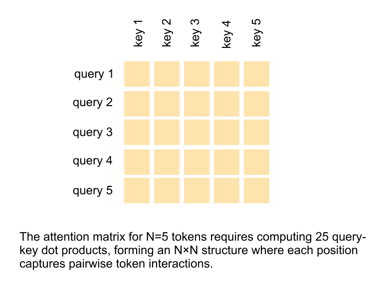
Figure 1.3 Global self attention in Vision Transformers.
For N input tokens, self attention computes an N × N matrix of query–key dot products, capturing all pairwise token interactions and leading to quadratic computational complexity.
Figure 1.4 illustrates this behavior with a concrete example. When image resolution is doubled along both spatial dimensions, the total number of pixels increases by a factor of four, but the attention computation increases by a factor of sixteen. This quadratic scaling makes Vision Transformers increasingly impractical for high resolution inputs. As a result, tasks that inherently require fine spatial detail, such as semantic segmentation or instance segmentation, become prohibitively expensive, limiting the applicability of vanilla Vision Transformers beyond image classification.
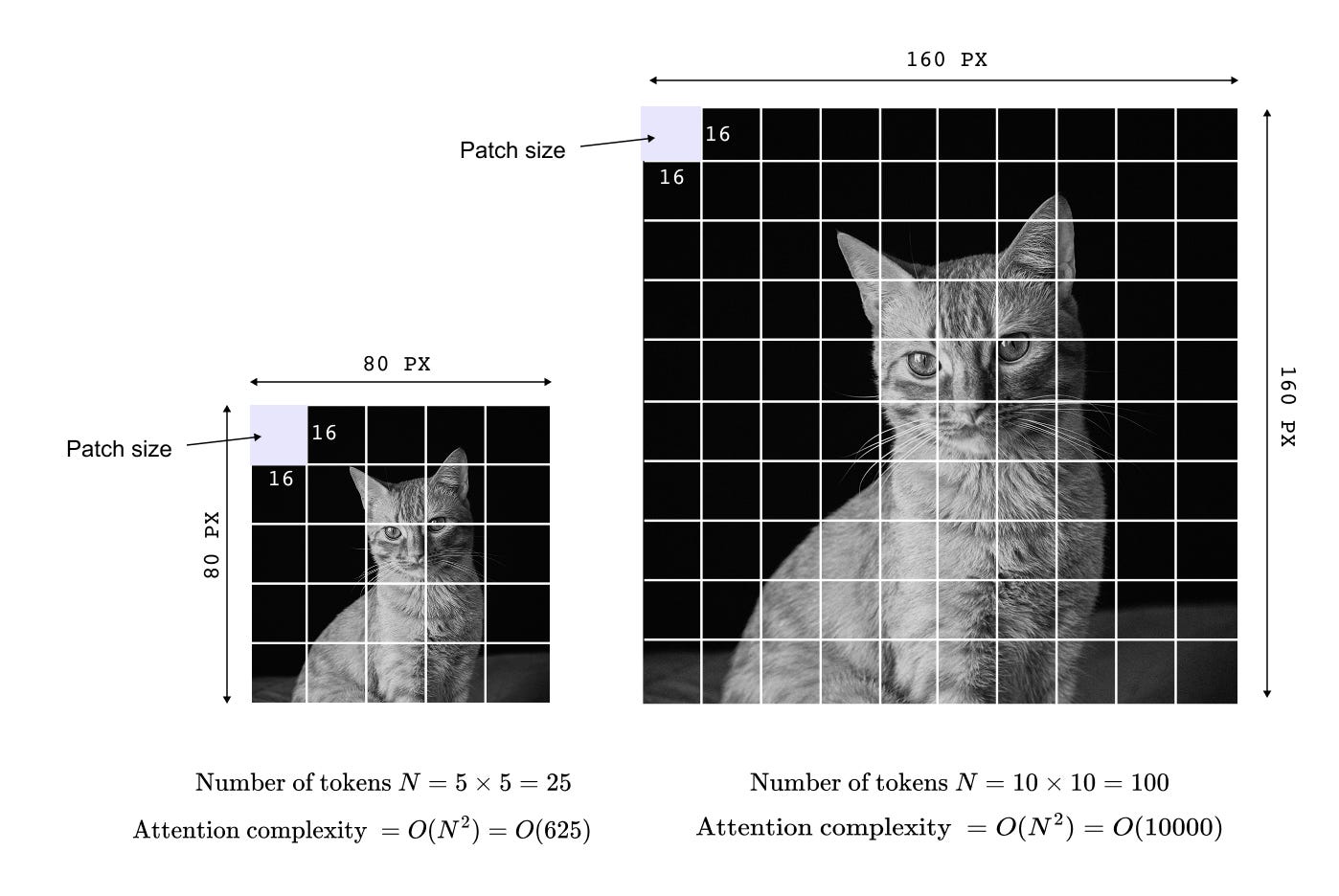
Figure 1.4 Quadratic complexity of global self attention in Vision Transformers.
Increasing image resolution leads to a quadratic growth in attention computation, as every patch token attends to every other token, making high resolution vision tasks computationally expensive.
1.3 Window Based Attention in Swin Transformers
Swin Transformers address the quadratic complexity of global self attention by restricting attention computation to local windows. Instead of allowing each patch token to attend to all other tokens in the image, attention is computed only among tokens that fall within a fixed size window. If each window contains M × M tokens, the attention cost within a window scales as O(M²), and since the number of windows grows linearly with image size, the overall complexity becomes linear with respect to the number of pixels.
This design dramatically improves scalability, but purely local attention introduces a new limitation. Tokens in different windows do not directly interact, which can restrict information flow across the image. Swin Transformers resolve this by introducing shifted window self attention. In alternating layers, the window partitioning is shifted spatially, allowing tokens that were previously in separate windows to attend to one another. Over multiple layers, this mechanism enables effective cross window communication while preserving linear computational complexity.
1.4 Hierarchical Feature Representation in Swin Transformers
Another key limitation of Vision Transformers is their flat representation structure. All transformer blocks operate on tokens derived from a single fixed patch size, resulting in a uniform spatial resolution throughout the network. This contrasts with convolutional architectures, which naturally build hierarchical feature representations by progressively reducing spatial resolution while increasing channel capacity.
Swin Transformers explicitly introduce a hierarchical architecture through patch merging stages. As shown in Figure 1.5, the model is organized into multiple stages, each operating at a different spatial scale. Early stages process high resolution features with fewer channels, while later stages operate on lower resolution representations with richer semantic content. This pyramid like structure closely aligns with the inductive biases of vision tasks and is particularly beneficial for dense prediction problems such as detection and segmentation.
By combining window based attention, shifted windows, and hierarchical feature construction, Swin Transformers bridge the gap between convolutional backbones and transformer based modeling. This design enables transformers to function as general purpose vision backbones, achieving strong performance across classification, object detection, and semantic segmentation tasks.
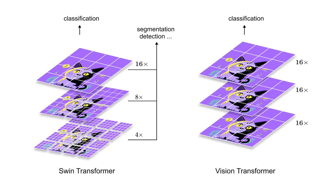
Figure 1.5 Hierarchical feature construction in Swin Transformers.
Spatial resolution is progressively reduced while channel dimensionality increases across stages, enabling multi scale feature representations similar to those used in convolutional architectures.
1.5 Overview of the Swin Transformer Architecture

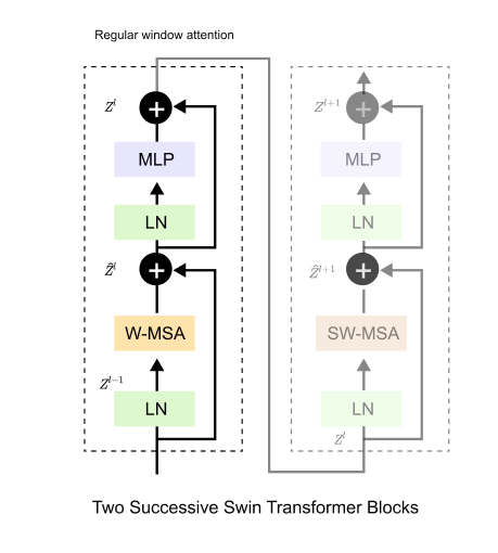
Figure 1.6 Swin Transformer architecture and block structure.
The model is composed of multiple stages with progressive resolution reduction and channel expansion. Each stage contains repeated Swin Transformer blocks, where window based and shifted window self attention are applied sequentially to enable efficient and scalable visual representation learning.
The Swin Transformer architecture is organized around two core ideas: staged hierarchical processing and localized self attention within transformer blocks. At a high level, the model is composed of multiple stages arranged sequentially, where each stage operates at a specific spatial resolution and feature dimensionality. The left portion of Figure 1.6 illustrates this overall architecture, showing how an input image is progressively transformed through a series of stages. Each stage consists of an embedding or patch merging operation followed by repeated Swin Transformer blocks. As the model advances through stages, spatial resolution is reduced while the number of feature channels increases, enabling increasingly abstract and semantically rich representations.
The fundamental computational unit of the architecture is the Swin Transformer block, expanded on the right side of Figure 1.6. A single Swin Transformer block is composed of two consecutive transformer style sub blocks. The first applies window based multi head self attention, where attention is computed independently within non overlapping local windows. The second applies shifted window based multi head self attention, which uses a spatially shifted window configuration to enable information exchange across neighboring windows. Each attention module is wrapped with layer normalization, residual connections, and a feed forward multilayer perceptron, closely mirroring the standard transformer design. While these components are individually familiar, their specific arrangement and interaction through windowing and shifting form the core novelty of the Swin architecture.
At this stage, several architectural questions naturally arise. How are patches grouped into windows, and how are windows constructed efficiently from the patch representation? How is positional information encoded without relying on absolute positional embeddings tied to a fixed token sequence? How exactly does window based attention differ from standard global attention, and how does the shifted window mechanism preserve cross window connectivity? Finally, how does this staged design give rise to hierarchical feature representations suitable for a wide range of vision tasks? These questions define the remainder of the Swin Transformer discussion and will be addressed step by step, beginning with the patching and window construction process in the next section.
1.6 Patch Partitioning and Linear Embedding
The first concrete operation applied to the input image in the Swin Transformer pipeline is patch partitioning. Given an RGB image of spatial resolution H×W with 3 channels, the image is divided into non overlapping square patches of size 4×4. This step is purely a reshaping operation and does not involve any learnable parameters. Each patch contains spatial information across all three color channels and serves as the atomic unit that will later be processed by transformer blocks.
Formally, partitioning the image into 4×4 patches produces a grid of patches along the height and width dimensions. The total number of patches is determined by the image resolution and patch size. Each patch is then flattened into a one dimensional vector by concatenating all pixel values within the patch across channels. Since each patch contains 4×4×3 values, the resulting vector has dimensionality 48. At this stage, the image is represented as a collection of vectors with shape
where each vector corresponds to a single spatial patch.
The patch partitioning process can be summarized as follows:
While these 48 dimensional vectors faithfully preserve all pixel level information within each patch, they are not yet suitable for transformer based processing. Transformers operate on tokens that share a common embedding dimension, typically denoted as C. To achieve this, each flattened patch vector is passed through a linear embedding layer, which performs a learned linear projection from 48 dimensions to C dimensions.
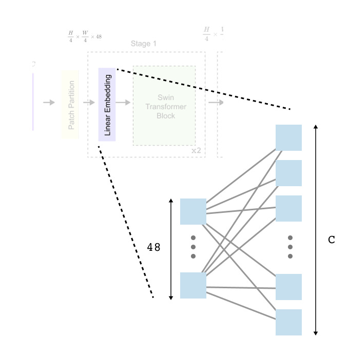
Figure 1.7 Patch partitioning and linear embedding in Swin Transformer.
The input image is divided into non overlapping 4×4 patches, each flattened into a 48 dimensional vector and linearly projected into a C dimensional embedding space before being processed by Swin Transformer blocks.
This linear embedding is equivalent to a fully connected layer applied independently to each patch. The transformation is parameterized by a weight matrix of shape 48×C , mapping each 1×48 patch vector to a 1×C embedding. After this step, all patches are represented in a common feature space, and the token dimensionality remains fixed throughout subsequent transformer blocks.
After linear embedding, the patch representation takes the form
which serves as the input to the first stage of Swin Transformer blocks. Importantly, neither patch partitioning nor linear embedding introduces any notion of attention or contextual interaction between patches. These steps strictly prepare the input representation and defer all contextual modeling to later stages of the architecture.
1.7 Patch Merging and Hierarchical Downsampling
Patch merging is the mechanism through which Swin Transformer transitions between stages and constructs hierarchical feature representations. Unlike patch partitioning, which operates directly on image pixels, patch merging operates on patch tokens produced by earlier stages. At the beginning of a stage, the feature map has spatial dimensions
with each token represented by a C-dimensional embedding. Patch merging reduces the number of tokens while increasing their representational capacity, closely mirroring the downsampling behavior observed in convolutional neural networks.
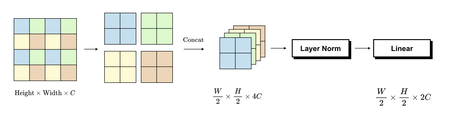
Figure 1.8 Patch merging operation in Swin Transformer.
Four neighboring patch tokens are concatenated along the channel dimension to form a 4C-dimensional representation, followed by a linear projection to 2C, reducing spatial resolution while increasing feature abstraction across stages.
The core operation in patch merging is the grouping of four neighboring patches arranged in a 2 × 2 grid. Consider four adjacent patch tokens, each of dimensionality C. These four tokens are concatenated along the channel dimension, producing a single token of dimensionality 4C. This operation reduces the spatial resolution by a factor of two along both height and width, since each 2 × 2 group of patches is replaced by a single patch token.
Concretely, if the input to patch merging has shape
then after concatenation of 2 × 2 neighboring patches, the intermediate representation becomes
At this point, the number of tokens has been reduced by a factor of four, but each token now aggregates information from a larger spatial region.
However, the Swin Transformer architecture does not propagate tokens with dimensionality 4C to the next stage. Instead, a linear projection is applied to each concatenated token to reduce the channel dimensionality from 4C to 2C. This projection is implemented as a fully connected layer shared across all tokens, analogous to the linear embedding used during initial patch embedding. As a result, the final output of patch merging has shape
This two step process can be summarized as follows:
Patch merging therefore performs two complementary roles simultaneously. First, it reduces spatial resolution, decreasing the number of tokens and improving computational efficiency for subsequent attention layers. Second, it increases feature abstraction by expanding the channel dimension before projecting it to a higher capacity embedding space. As this operation is repeated across stages, the model progressively moves from fine grained local representations to coarser, more semantic features. This progressive reduction in token count and increase in feature dimensionality is the foundation of the hierarchical structure that enables Swin Transformer to serve as a general purpose vision backbone.
1.8 Attention Complexity in Swin Transformers
The primary motivation behind the Swin Transformer design is to address the quadratic attention complexity of standard Vision Transformers while preserving the expressive power of self attention. This is achieved by restricting self attention computation to local windows instead of the entire image.
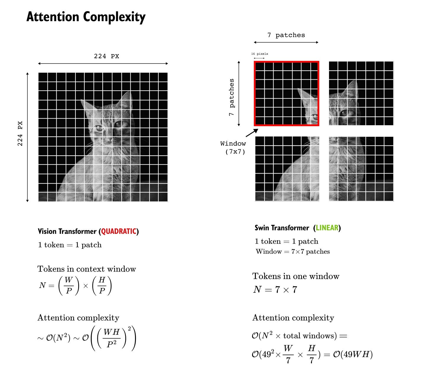
Figure 1.9 Attention complexity comparison between Vision Transformer and Swin Transformer.
Vision Transformer computes global self attention over all patches, resulting in quadratic complexity with respect to image size. Swin Transformer restricts attention to fixed size local windows, leading to linear scaling while preserving local contextual modeling.
Consider an input image of spatial resolution H×W, divided into non overlapping patches of size P×P. As before, each patch is treated as a token. The total number of patches in the image is therefore
In a Vision Transformer, all N_patches tokens participate in global self attention, leading to quadratic complexity. Swin Transformer alters this computation by introducing fixed size windows.
Attention Computation Within a Single Window
In Swin Transformer, attention is computed locally within windows of size M×M patches. For a single window, the number of tokens is
Since self attention computes all pairwise interactions between queries and keys, the attention complexity for one window is
This cost is independent of the overall image resolution and depends only on the window size.
Number of Windows in the Image
To compute the total attention cost, we must account for how many such windows exist in the image.
The number of patches along height and width are
Each window spans M patches along each spatial dimension. Therefore, the number of windows along height and width are
The total number of windows in the image is
Total Attention Complexity
The total attention complexity for the entire image is obtained by multiplying the cost per window with the total number of windows
Since M and P are fixed hyperparameters, the dominant scaling term is HW. Thus, the overall attention complexity scales linearly with the number of image pixels
This is in contrast to the Vision Transformer, where attention complexity scales as
By limiting self attention to local windows, Swin Transformer converts quadratic global attention into linear attention with respect to image size. As image resolution increases, the attention cost grows proportionally rather than quadratically, making Swin Transformer far more suitable for high resolution vision tasks.
1.9 Shifted Windows for Long Range Interaction in Swin Transformer
Window based self attention significantly reduces computational cost by restricting attention to local regions. However, this restriction introduces an important limitation: patches that are spatially close but lie in different windows cannot attend to each other. Swin Transformer resolves this limitation using the idea of shifted windows, which enables information flow across window boundaries while preserving linear complexity.
1.9.1 Limitation of Regular Non Overlapping Windows
In regular window based self attention, the image is first partitioned into non overlapping patches. These patches are then grouped into non overlapping windows of fixed size.
Let H and W denote image height and width in pixels P denote patch size in pixels M denote window size in number of patches per side
Each window contains
tokens, and self attention is computed only within these tokens.
As a result, attention between any two patches is allowed if and only if both patches belong to the same window.
This creates a hard boundary:
• Patches A and B may be geometrically adjacent but have zero attention if they fall in different windows
• Patches A and C may be far apart but can attend if they share a window
Thus, attention is governed by window membership, not spatial proximity.
1.9.2 Why Regular Windows Are Insufficient
Because attention is restricted to fixed windows:
• Local context is well captured
• Global and cross window dependencies are missing
This is problematic for vision tasks where objects often span across window boundaries. Simply enlarging the window would increase computation and defeat the purpose of window based attention.
Swin Transformer solves this using alternating regular and shifted window attention blocks.
1.9.3 Shifted Window Mechanism
In the shifted window block, window boundaries are shifted by half the window size along both height and width.
This shift changes window assignments without changing patch content.
As a result:
• Patches that were previously in different windows are now grouped together
• New attention connections are formed across previous window boundaries
Importantly, this shift does not introduce overlapping attention computation. Each block still computes attention within fixed size windows.
1.9.4 Cyclic Shifting to Preserve Window Structure
A naive shift creates incomplete windows near image boundaries, leading to uneven window sizes. Padding could fix this, but padding introduces unnecessary computation and irregular window sizes.
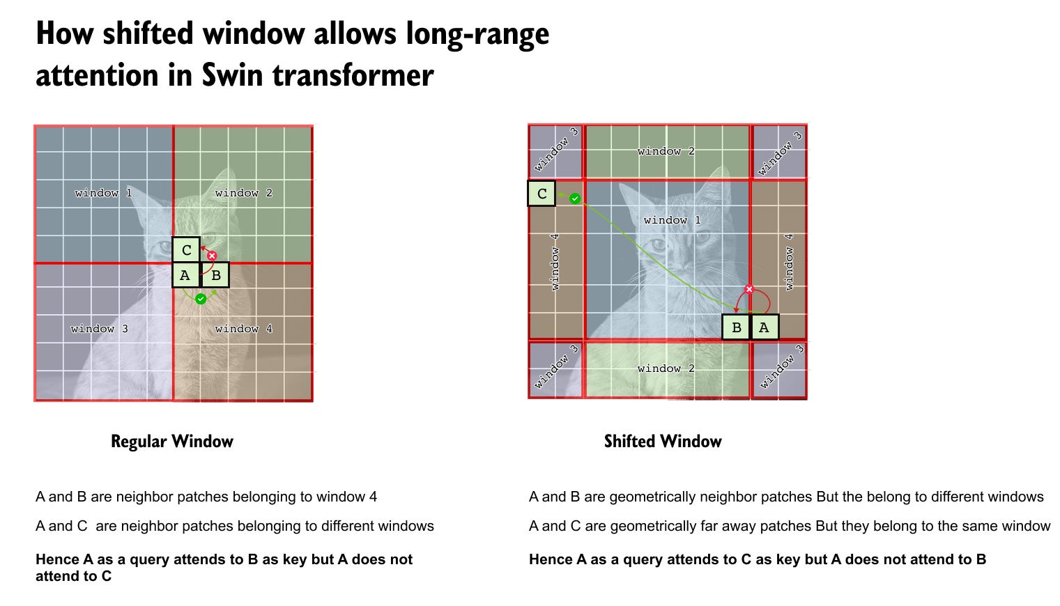
Figure 1.10 Shifted window attention in Swin Transformer.
Regular window attention restricts interactions to fixed non overlapping windows, preventing neighboring patches across window boundaries from attending to each other. Shifted windows reassign patches to new windows using cyclic shifting, enabling cross window and long range interactions across consecutive transformer blocks while preserving linear attention complexity.
Instead, Swin Transformer uses cyclic shifting.
Cyclic shifting works as follows:
• Patches that move out of the image on one side re enter from the opposite side
• Only window indices are shifted, not pixel values
• Each shifted window still contains exactly M × M patches
This mechanism is equivalent to rolling the image on a torus or cylinder.
As a result:
• All windows remain uniform in size
• Attention computation remains efficient
• No padding overhead is introduced
1.9.5 How Shifted Windows Enable Long Range Attention
Consider two consecutive transformer blocks operating in sequence: a regular window attention block followed by a shifted window attention block.(as illustrated in Figure 1.10) In the first block, self attention is strictly confined to non overlapping local windows, which limits interactions to patches that share the same window. In the subsequent block, the window partitioning is shifted, causing patches to be regrouped into different windows. As a result, patches that were previously unable to attend to each other due to window boundaries are now placed within the same window and can directly interact. Across these two blocks, information propagates across neighboring windows, and with repeated stacking of such block pairs, progressively longer range dependencies are established. Consequently, Swin Transformer achieves effective global context modeling indirectly, without ever computing full global self attention.
Swin Transformer does not allow every patch to attend to every other patch in a single layer. Instead, it enables long range dependency through alternating locality patterns across layers, while maintaining linear computational complexity with respect to image size.
1.10 Window-Based Self-Attention with Relative Position Bias and Masking
In Swin Transformer, positional information and locality constraints are integrated directly into the self attention computation rather than being handled as a preprocessing step. This design choice is tightly coupled with window based attention and is essential for maintaining linear computational complexity while preserving spatial structure. Each transformer stage alternates between blocks that use regular window attention and blocks that use shifted window attention, and the attention formulation is adapted accordingly.
We first consider the case of regular window attention. In this setting, the feature map is partitioned into non overlapping windows of fixed size, and self attention is computed independently within each window. Let qi and kj denote the query and key vectors corresponding to patches i and j within the same window, and let d be the head dimension. The attention weight α_ij is computed as
where b_ij is a learnable relative position bias term. This bias depends only on the relative spatial offset between patches i and j within the window, not on their absolute positions in the image. Unlike Vision Transformers, which add positional embeddings to token representations before entering the transformer blocks, Swin Transformer injects positional information directly into the attention logits. This allows the model to encode spatial relationships locally and naturally aligns with the window based formulation. Since all query key pairs belong to the same window in this block, no additional constraints are required, and attention is computed over all patch pairs within the window.
The situation changes in the shifted window attention block. Here, the window partition is shifted by half the window size along both height and width to enable information flow across neighboring windows. After shifting, a single shifted window may contain patches that originate from different regular windows. If attention were computed using the same formulation as above, patches that should not interact would incorrectly attend to each other. To prevent this, Swin Transformer introduces an additive attention mask term.
In the shifted window block, the attention weight is computed as
The mask term mask_ij enforces window locality after shifting. If patches i and j belong to the same window after shifting, the mask value is zero,
and attention between them is allowed. If they belong to different windows, the mask value is set to negative infinity,
Because the mask is added before the softmax operation, any attention score associated with −∞ is driven to zero after normalization. This guarantees that patches from different windows do not attend to each other, even though they may be present within the same shifted window tensor. Importantly, this masking operation is additive and should not be confused with multiplicative masking or dropout. It is a precise mathematical mechanism that preserves the structure of window based attention under shifting.
Together, relative position bias and attention masking form the core of Swin Transformer’s window based self attention. Relative position bias provides fine grained spatial awareness within each window, while masking ensures that attention remains well defined and localized in the shifted window configuration. By alternating regular and shifted window attention blocks, Swin Transformer enables information to propagate across windows over depth, gradually building long range dependencies without ever computing full global self attention. This formulation is a key reason why Swin Transformer achieves strong performance while maintaining linear scaling with respect to image size.
1.11 Relative Position Bias Parameterization in Swin Transformer
An important detail in Swin Transformer is how relative position bias is parameterized and shared across attention heads. Unlike absolute positional embeddings, which require a unique embedding for every spatial location, relative position bias depends only on the relative offset between two patches inside a window. This makes the formulation independent of absolute image size and naturally compatible with window-based attention.
For a window of size M×M, the relative displacement between two patches along height and width can take values in the range
This results in a total of
unique relative position offsets. Swin Transformer maintains a learnable bias table of this size for each attention head. During attention computation, each query–key pair (i,j) indexes into this table based on their relative spatial displacement, and the corresponding scalar bias is added to the attention logit.
This design has several advantages. First, it significantly reduces the number of learnable positional parameters compared to absolute embeddings. Second, it allows the same bias table to be reused across all windows within a layer, enforcing translation equivariance. Finally, because the bias depends only on relative offsets, it generalizes naturally to different image sizes at inference time.
1.12 Absence of Class Token in Swin Transformer
Another notable departure from the original Vision Transformer design is the absence of a dedicated class token in Swin Transformer. In Vision Transformers, a special learnable token is prepended to the patch sequence and used as the global image representation for classification tasks. This approach assumes global self attention, where the class token can attend to all patches in a single layer.
In Swin Transformer, attention is localized within windows, and no single token has access to all patches in one layer. As a result, a class token would not be able to aggregate global information efficiently. Instead, Swin Transformer relies on hierarchical feature aggregation to build global representations.
For image classification, the final stage of the network produces a low-resolution feature map with rich semantic content. Global average pooling is applied over the spatial dimensions to aggregate information across all remaining tokens. The pooled representation is then passed to a classification head. This approach aligns closely with convolutional architectures and avoids introducing a special token that does not naturally fit the window-based attention paradigm.
1.13 Output Heads and Task Generalization
One of the strengths of Swin Transformer is its flexibility as a general-purpose vision backbone. The hierarchical feature maps produced at different stages can be directly reused for a wide range of downstream tasks.
For image classification, only the final stage output is used, followed by global pooling and a linear classifier. For object detection and instance segmentation, intermediate feature maps from multiple stages are extracted and fed into feature pyramid networks or task-specific heads. For semantic segmentation, high-resolution features from early stages and semantically rich features from deeper stages are combined to produce dense predictions.
This multi-scale output capability is a direct consequence of the hierarchical design introduced by patch merging. Unlike flat Vision Transformers, Swin Transformer naturally exposes feature representations at multiple resolutions, making it particularly well suited for dense prediction tasks.
1.14 Comparison with Convolutional Backbones
Although Swin Transformer is built entirely using transformer blocks, its architectural philosophy closely mirrors that of convolutional neural networks. Locality is enforced through window-based attention, hierarchical feature representations are constructed via patch merging, and translation equivariance is preserved through relative position bias and weight sharing across windows.
At the same time, Swin Transformer retains the key advantages of transformers, including dynamic content-dependent receptive fields and the ability to model long-range dependencies through depth. The shifted window mechanism effectively replaces the role of increasing convolutional kernel sizes or dilated convolutions, enabling cross-region interaction without sacrificing efficiency.
This hybridization of transformer flexibility with convolutional inductive biases is a central reason for Swin Transformer’s strong empirical performance across diverse vision benchmarks.
1.15 Concluding Remarks on Swin Transformer
Swin Transformer represents a significant step forward in adapting transformer architectures to the unique demands of visual data. By replacing global self attention with window-based attention and introducing shifted windows for cross-region communication, it resolves the fundamental scalability limitations of Vision Transformers while preserving their expressive capacity.
The introduction of hierarchical feature representations through patch merging aligns the model with long-standing principles of visual processing, enabling seamless integration into detection, segmentation, and recognition pipelines. Relative position bias provides an elegant and efficient mechanism for encoding spatial relationships, while attention masking ensures correctness under window shifting.
Rather than computing global context in a single layer, Swin Transformer builds global understanding gradually through depth, leveraging alternating locality patterns across layers. This design demonstrates that effective global reasoning does not require global computation at every step.
As a result, Swin Transformer serves not only as a powerful architecture in its own right, but also as a blueprint for future vision transformers that balance efficiency, scalability, and representational strength.
Watch the full lecture video here
If you would like to deepen your understanding of Swin Transformer and see these ideas explained visually and intuitively, you can refer to the accompanying video linked above. If you wish to get access to our code files, handwritten notes, all lecture videos, Discord channel, and other PDF handbooks that we have compiled, along with a code certificate at the end of the program, you can consider being part of the pro version of the “Transformers for Vision Bootcamp”. You will find the details here:
https://vision-transformer.vizuara.ai/
Other resources
If you like this content, please check out our research bootcamps on the following topics:
CV: https://cvresearchbootcamp.vizuara.ai/
GenAI: https://flyvidesh.online/gen-ai-professional-bootcamp
RL: https://rlresearcherbootcamp.vizuara.ai/
SciML: https://flyvidesh.online/ml-bootcamp
ML-DL: https://flyvidesh.online/ml-dl-bootcamp
Connect with us
Dr. Sreedath Panat
LinkedIn : https://www.linkedin.com/in/sreedath-panat/
Twitter/X : https://x.com/sreedathpanat
Mayank Pratap Singh
LinkedIn : www.linkedin.com/in/mayankpratapsingh022
Twitter/X : x.com/Mayank_022