𝗨𝗻𝗱𝗲𝗿𝘀𝘁𝗮𝗻𝗱𝗶𝗻𝗴 𝗟𝗼𝗴𝗶𝘀𝘁𝗶𝗰 𝗥𝗲𝗴𝗿𝗲𝘀𝘀𝗶𝗼𝗻 𝗧𝗵𝗿𝗼𝘂𝗴𝗵 𝗔𝗻𝗶𝗺𝗮𝘁𝗶𝗼𝗻

Visualizing complex concepts makes them easier to grasp, and logistic regression is no exception! This animation provides an intuitive way to understand how logistic regression learns through gradient descent.

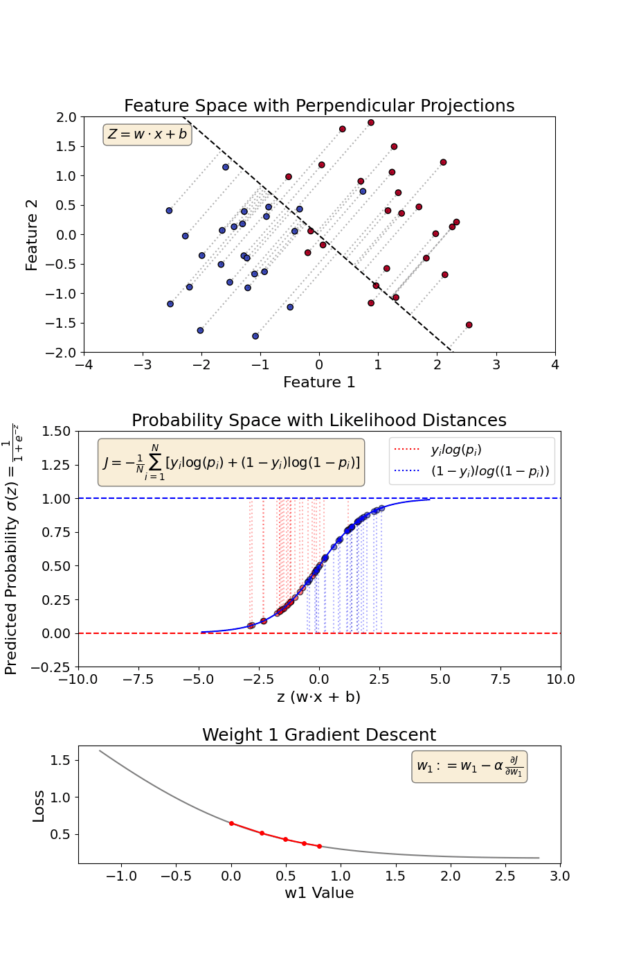
🔹 𝗞𝗲𝘆 𝗧𝗮𝗸𝗲𝗮𝘄𝗮𝘆𝘀 𝗳𝗿𝗼𝗺 𝘁𝗵𝗲 𝗔𝗻𝗶𝗺𝗮𝘁𝗶𝗼𝗻:

𝟭. 𝗙𝗲𝗮𝘁𝘂𝗿𝗲 𝗦𝗽𝗮𝗰𝗲 & 𝗗𝗲𝗰𝗶𝘀𝗶𝗼𝗻 𝗕𝗼𝘂𝗻𝗱𝗮𝗿𝘆 (𝗚𝗿𝗮𝗽𝗵 𝟭)

✔️ The value of 𝗭 is determined by the 𝗽𝗲𝗿𝗽𝗲𝗻𝗱𝗶𝗰𝘂𝗹𝗮𝗿 𝗱𝗶𝘀𝘁𝗮𝗻𝗰𝗲 between a data point and the decision boundary.

✔️ With each 𝗴𝗿𝗮𝗱𝗶𝗲𝗻𝘁 𝗱𝗲𝘀𝗰𝗲𝗻𝘁 𝘀𝘁𝗲𝗽, the decision boundary shifts, and Z progressively increases.

𝟮. 𝗣𝗿𝗼𝗯𝗮𝗯𝗶𝗹𝗶𝘁𝘆 & 𝗦𝗶𝗴𝗺𝗼𝗶𝗱 𝗙𝘂𝗻𝗰𝘁𝗶𝗼𝗻 (𝗚𝗿𝗮𝗽𝗵 𝟮)

✔️ Z is used to compute the 𝗽𝗿𝗲𝗱𝗶𝗰𝘁𝗲𝗱 𝗽𝗿𝗼𝗯𝗮𝗯𝗶𝗹𝗶𝘁𝘆 via the 𝘀𝗶𝗴𝗺𝗼𝗶𝗱 𝗳𝘂𝗻𝗰𝘁𝗶𝗼𝗻.

✔️ As Z increases, the model becomes more confident in its classifications, increasing the likelihood of correct predictions.

𝟯. 𝗚𝗿𝗮𝗱𝗶𝗲𝗻𝘁 𝗗𝗲𝘀𝗰𝗲𝗻𝘁 & 𝗪𝗲𝗶𝗴𝗵𝘁 𝗨𝗽𝗱𝗮𝘁𝗲𝘀 (𝗚𝗿𝗮𝗽𝗵 𝟯)

✔️ Gradient descent 𝘂𝗽𝗱𝗮𝘁𝗲𝘀 𝘁𝗵𝗲 𝘄𝗲𝗶𝗴𝗵𝘁𝘀 iteratively to minimize the loss function.

✔️ This process 𝘀𝗵𝗶𝗳𝘁𝘀 𝘁𝗵𝗲 𝗱𝗲𝗰𝗶𝘀𝗶𝗼𝗻 𝗯𝗼𝘂𝗻𝗱𝗮𝗿𝘆 in the feature space, refining classification over time.

By animating these fundamental steps, we can clearly observe 𝗵𝗼𝘄 𝗹𝗼𝗴𝗶𝘀𝘁𝗶𝗰 𝗿𝗲𝗴𝗿𝗲𝘀𝘀𝗶𝗼𝗻 𝗼𝗽𝘁𝗶𝗺𝗶𝘇𝗲𝘀 𝗶𝘁𝘀 𝗱𝗲𝗰𝗶𝘀𝗶𝗼𝗻 𝗯𝗼𝘂𝗻𝗱𝗮𝗿𝘆.

For more AI and machine learning insights, check out 𝗩𝗶𝘇𝘂𝗿𝗮’𝘀 𝗔𝗜 𝗡𝗲𝘄𝘀𝗹𝗲𝘁𝘁𝗲𝗿: https://www.vizuaranewsletter.com?r=502twn.

For a detailed understanding, check out these videos:

1️⃣ 𝗟𝗼𝗴𝗶𝘀𝘁𝗶𝗰 𝗥𝗲𝗴𝗿𝗲𝘀𝘀𝗶𝗼𝗻 𝗦𝗶𝗺𝗽𝗹𝗶𝗳𝗶𝗲𝗱: Your First Step into Classification | Intuitive Approach:

2️⃣ 𝗟𝗼𝘀𝘀 𝗙𝘂𝗻𝗰𝘁𝗶𝗼𝗻 𝗳𝗼𝗿 𝗟𝗼𝗴𝗶𝘀𝘁𝗶𝗰 𝗥𝗲𝗴𝗿𝗲𝘀𝘀𝗶𝗼𝗻 | Negative Log Likelihood | Log(Odds) | Sigmoid: