Adam- The most famous ML optimizer from Scratch

With a recap of vanilla/normal/batch gradient descent

Optimization in machine learning is all about finding that sweet spot—a set of parameters that minimizes error. While Gradient Descent laid the foundation for this, its practical limitations called for upgrade. Adam optimizer is the most popular optimizers. In this article we will discuss what is Adam optimizer and why is it a big deal. We will also implement Adam from scratch at the end of this article.

A quick recap on vanilla gradient descent

Recap of Gradient Descent and Its Shortcomings

What Is Gradient Descent?

Gradient Descent is an iterative optimization algorithm used to minimize a loss function L(θ). At each step, it updates the model parameters θ by moving in the direction opposite to the gradient of the loss function with respect to θ:

\(\theta = \theta - \eta \nabla L(\theta) \)

Here:

• ∇L(θ): Gradient of the loss function.

• η: Learning rate (step size).

Key Properties:

1. It computes the gradient over the entire dataset at each step.

2. Guarantees a smooth and steady descent towards the minimum of L(θ)

The Struggles of Vanilla Gradient Descent

1. Computational Overhead: Calculating the gradient over the entire dataset is computationally expensive for large datasets.

   • Example: For a dataset with N samples, computing the gradient requires N operations per update.

2. Slow Convergence: Gradient Descent can take small, steady steps and struggle with large datasets or complex loss landscapes.

3. Local Minima or Saddle Points: It may get stuck in a local minimum or wander in a flat saddle region, delaying convergence.

These limitations led to the development of Stochastic Gradient Descent, which makes optimization faster and more flexible.

NOTE: The “normal” gradient descent is also called as vanilla gradient descent or batch gradient descent (BGD). Batch because the parameter update is calculated with respect to all data points in the batch.

Adam Optimizer: The King of Gradient Descent Methods

If optimization were a competition, the Adam optimizer would be royalty—balancing speed, stability, and adaptability like no other. It’s one of the most widely used algorithms in deep learning, praised for its ability to handle noisy gradients, sparse data, and complex optimization landscapes. But what makes Adam so special? In this article, we’ll explore how Adam works, its mathematical foundations, and why it’s often the first choice for training machine learning models.

Comparison of Optimization Paths: Gradient Descent vs. Adam. This plot illustrates the optimization trajectories for Gradient Descent (blue) and Adam (orange) on a 2D loss surface. Gradient Descent struggles with oscillations in narrow valleys, leading to slower convergence, while Adam smoothly adjusts its path, leveraging adaptive learning rates and momentum to converge efficiently. Start and end points for each optimizer are marked for clarity.

The Evolution of Optimization Algorithms

Let’s set the stage. In machine learning, the goal of optimization is to minimize a loss function by iteratively adjusting model parameters. Algorithms like Gradient Descent, Momentum, and RMSprop have laid the foundation for this, each improving on its predecessor.

1. Gradient Descent: Updates parameters in the direction of the steepest descent but struggles with slow convergence and uniform learning rates.

2. Momentum: Introduces a velocity term to smooth updates and accelerate convergence.

3. RMSprop: Adapts the learning rate for each parameter by normalizing gradients, tackling challenges like exploding or vanishing gradients.

Adam (short for Adaptive Moment Estimation) combines the best of Momentum and RMSprop to create a robust, adaptive optimization algorithm that works well out of the box.

How Does Adam Work?

Adam uses two key ideas:

1. Momentum: Keeps track of an exponentially decaying moving average of past gradients to smooth updates.

2. Adaptive Learning Rates: Scales each parameter’s updates using a running average of the squared gradients, ensuring stable and efficient convergence.

Here’s the step-by-step breakdown:

1. Momentum Term (First Moment Estimate)

Adam calculates an exponentially decaying average of past gradients:

\(m_t = \beta_1 m_{t-1} + (1 - \beta_1) g_t \)

Where:

• mt​: First moment estimate (essentially the velocity).

• gt​: Gradient of the loss function at time t.

• β1​: Decay rate for the first moment (commonly 0.9).

This term (mt) helps smooth updates by accumulating gradient history.

2. RMS Term (Second Moment Estimate)

Adam also maintains a moving average of the squared gradients:

\(v_t = \beta_2 v_{t-1} + (1 - \beta_2) g_t^2 \)

Where:

• vt​: Second moment estimate (variance of gradients).

• β2​: Decay rate for the second moment (commonly 0.999).

This term adapts the learning rate for each parameter based on the magnitude of the gradients, preventing excessively large updates.

3. Bias Correction

To counteract the bias introduced by initializing mt​ and vt to zero, Adam applies a correction:

\(\hat{m}_t = \frac{m_t}{1 - \beta_1^t}, \quad \hat{v}_t = \frac{v_t}{1 - \beta_2^t} \)

This ensures that mt​ and vt accurately reflect the gradients, especially in early iterations.

4. Parameter Update

Finally, Adam updates the parameters:

\(\theta = \theta - \frac{\eta}{\sqrt{\hat{v}_t} + \epsilon} \hat{m}_t \)

Where:

• η: Learning rate (commonly 0.001).

• ϵ: A small value (e.g., 10−^-8) to prevent division by zero.

Why Adam Is So Popular

Adam’s clever combination of momentum and adaptive learning rates gives it several key advantages:

1. Fast Convergence: Adam combines the acceleration of Momentum with the stability of RMSprop, leading to faster convergence on most problems.

2. Adaptive Learning Rates: Each parameter’s updates are scaled individually, making Adam effective for problems with sparse gradients or varying scales.

3. Noise Resilience: Adam handles noisy or non-stationary gradients well, making it ideal for deep learning tasks.

4. Minimal Tuning: With default hyperparameters (β1=0.9,β2=0.999,η=0.001), Adam works well across a wide range of models and datasets.

Limitations of Adam

While Adam is versatile, it’s not without flaws:

1. Over-Adaptation: In some cases, Adam’s adaptability can lead to overfitting or poor generalization.

2. Suboptimal Convergence: For certain problems, Adam may converge to a suboptimal solution compared to simpler algorithms like SGD.

3. Learning Rate Sensitivity: Despite being adaptive, Adam’s performance can be sensitive to the initial learning rate η.

Where Adam Shines

Adam is particularly effective in:

• Deep Learning: It’s the go-to optimizer for training deep neural networks, including convolutional and recurrent architectures.

• Sparse Gradients: Tasks like natural language processing or recommendation systems often have sparse updates, where Adam excels.

• Noisy Gradients: Adam handles complex optimization landscapes and stochastic environments gracefully.

Code implementation of Adam v/s Vanilla Gradient Descent

import numpy as np
import matplotlib.pyplot as plt

def quadratic_loss(x, y):
    return x**2 + 10 * y**2

def quadratic_grad(x, y):
    dx = 2 * x
    dy = 20 * y
    return np.array([dx, dy])

def gradient_descent(grad_func, lr, epochs, start_point):
    x, y = start_point
    path = [(x, y)]
    losses = [quadratic_loss(x, y)]

    for _ in range(epochs):
        grad = grad_func(x, y)
        x -= lr * grad[0]
        y -= lr * grad[1]
        path.append((x, y))
        losses.append(quadratic_loss(x, y))

    return np.array(path), losses


def adam_optimizer(grad_func, lr, beta1, beta2, epsilon, epochs, start_point):
    x, y = start_point
    m = np.array([0.0, 0.0])  # First moment (Momentum)
    v = np.array([0.0, 0.0])  # Second moment (RMSProp)
    path = [(x, y)]
    losses = [quadratic_loss(x, y)]

    for t in range(1, epochs + 1):
        grad = grad_func(x, y)  # Compute gradients

        # Update biased first moment estimate
        m = beta1 * m + (1 - beta1) * grad

        # Update biased second moment estimate
        v = beta2 * v + (1 - beta2) * (grad ** 2)

        # Bias correction
        m_hat = m / (1 - beta1 ** t)
        v_hat = v / (1 - beta2 ** t)

        # Update parameters
        x -= lr * m_hat[0] / (np.sqrt(v_hat[0]) + epsilon)
        y -= lr * m_hat[1] / (np.sqrt(v_hat[1]) + epsilon)

        path.append((x, y))
        losses.append(quadratic_loss(x, y))

    return np.array(path), losses

def plot_paths(function, paths, labels, title):
    X, Y = np.meshgrid(np.linspace(-2, 2, 400), np.linspace(-2, 2, 400))
    Z = function(X, Y)

    plt.figure(figsize=(8, 6))
    plt.contour(X, Y, Z, levels=50, cmap='jet')

    for path, label in zip(paths, labels):
        plt.plot(path[:, 0], path[:, 1], label=label)
        plt.scatter(path[0, 0], path[0, 1], color='green', label="Start")
        plt.scatter(path[-1, 0], path[-1, 1], color='red', label="End")

    plt.title(title)
    plt.xlabel("x")
    plt.ylabel("y")
    plt.legend()
    plt.show()

def plot_losses(losses, labels, title):
    plt.figure(figsize=(8, 6))

    for loss, label in zip(losses, labels):
        plt.plot(loss, label=label)

    plt.title(title)
    plt.xlabel("Epoch")
    plt.ylabel("Loss")
    plt.legend()
    plt.show()

lr_gd = 0.2  # Learning rate for GD
lr_adam = 0.2  # Learning rate for Adam
beta1 = 0.9  # Beta1 for Adam
beta2 = 0.999  # Beta2 for Adam
epsilon = 1e-8  # Small constant for Adam
epochs = 550
start_point = (1.5, 1.5)  # Initial point far from the minimum

path_gd, losses_gd = gradient_descent(quadratic_grad, lr_gd, epochs, start_point)
path_adam, losses_adam = adam_optimizer(quadratic_grad, lr_adam, beta1, beta2, epsilon, epochs, start_point)

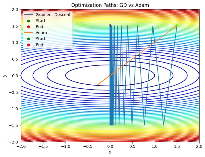
plot_paths(quadratic_loss, [path_gd, path_adam],
           ["Gradient Descent", "Adam"],
           "Optimization Paths: GD vs Adam")

plot_losses([losses_gd, losses_adam],
            ["Gradient Descent", "Adam"],
            "Loss vs Epochs: GD vs Adam")

import numpy as np
import matplotlib.pyplot as plt

# Define a quadratic loss function
# Loss function: f(x, y) = x^2 + 10*y^2 (steep valley along y-axis)
def quadratic_loss(x, y):
    return x**2 + 10 * y**2

# Gradient of the loss function
def quadratic_grad(x, y):
    dx = 2 * x
    dy = 20 * y
    return np.array([dx, dy])

# Momentum Optimizer
def momentum_optimizer(grad_func, lr, beta, epochs, start_point):
    x, y = start_point
    v = np.array([0.0, 0.0])  # Initialize velocity
    path = [(x, y)]
    losses = [quadratic_loss(x, y)]

    for _ in range(epochs):
        grad = grad_func(x, y)
        v = beta * v + (1 - beta) * grad  # Update velocity
        x -= lr * v[0]  # Update x
        y -= lr * v[1]  # Update y

        path.append((x, y))
        losses.append(quadratic_loss(x, y))

    return np.array(path), losses

# Adam Optimizer
def adam_optimizer(grad_func, lr, beta1, beta2, epsilon, epochs, start_point):
    x, y = start_point
    m = np.array([0.0, 0.0])  # First moment (Momentum)
    v = np.array([0.0, 0.0])  # Second moment (RMSProp)
    path = [(x, y)]
    losses = [quadratic_loss(x, y)]

    for t in range(1, epochs + 1):
        grad = grad_func(x, y)  # Compute gradients

        # Update biased first moment estimate
        m = beta1 * m + (1 - beta1) * grad

        # Update biased second moment estimate
        v = beta2 * v + (1 - beta2) * (grad ** 2)

        # Bias correction
        m_hat = m / (1 - beta1 ** t)
        v_hat = v / (1 - beta2 ** t)

        # Update parameters
        x -= lr * m_hat[0] / (np.sqrt(v_hat[0]) + epsilon)
        y -= lr * m_hat[1] / (np.sqrt(v_hat[1]) + epsilon)

        path.append((x, y))
        losses.append(quadratic_loss(x, y))

    return np.array(path), losses

# Visualization of paths
def plot_paths(function, paths, labels, title):
    X, Y = np.meshgrid(np.linspace(-2, 2, 400), np.linspace(-2, 2, 400))
    Z = function(X, Y)

    plt.figure(figsize=(8, 6))
    plt.contour(X, Y, Z, levels=50, cmap='jet')

    for path, label in zip(paths, labels):
        plt.plot(path[:, 0], path[:, 1], label=label)
        plt.scatter(path[0, 0], path[0, 1], color='green', label="Start")
        plt.scatter(path[-1, 0], path[-1, 1], color='red', label="End")

    plt.title(title)
    plt.xlabel("x")
    plt.ylabel("y")
    plt.legend()
    plt.show()

# Visualization of losses
def plot_losses(losses, labels, title):
    plt.figure(figsize=(8, 6))

    for loss, label in zip(losses, labels):
        plt.plot(loss, label=label)

    plt.title(title)
    plt.xlabel("Epoch")
    plt.ylabel("Loss")
    plt.legend()
    plt.show()

# Parameters
lr_momentum = 0.1  # Learning rate for Momentum
lr_adam = 0.1  # Learning rate for Adam
beta1 = 0.9  # Beta1 for Adam
beta2 = 0.999  # Beta2 for Adam
beta_momentum = 0.9  # Momentum coefficient
epsilon = 1e-8  # Small constant for Adam
epochs = 100
start_point = (1.5, 1.5)  # Initial point far from the minimum

# Run optimizations
path_momentum, losses_momentum = momentum_optimizer(quadratic_grad, lr_momentum, beta_momentum, epochs, start_point)
path_adam, losses_adam = adam_optimizer(quadratic_grad, lr_adam, beta1, beta2, epsilon, epochs, start_point)

# Plot results
plot_paths(quadratic_loss, [path_momentum, path_adam],
           ["Momentum", "Adam"],
           "Optimization Paths: Momentum vs Adam")

plot_losses([losses_momentum, losses_adam],
            ["Momentum", "Adam"],
            "Loss vs Epochs: Momentum vs Adam")

Code for Adam vs momentum comparison

import numpy as np
import matplotlib.pyplot as plt

# Define a quadratic loss function
# Loss function: f(x, y) = x^2 + 10*y^2 (steep valley along y-axis)
def quadratic_loss(x, y):
    return x**2 + 10 * y**2

# Gradient of the loss function
def quadratic_grad(x, y):
    dx = 2 * x
    dy = 20 * y
    return np.array([dx, dy])

# Momentum Optimizer
def momentum_optimizer(grad_func, lr, beta, epochs, start_point):
    x, y = start_point
    v = np.array([0.0, 0.0])  # Initialize velocity
    path = [(x, y)]
    losses = [quadratic_loss(x, y)]

    for _ in range(epochs):
        grad = grad_func(x, y)
        v = beta * v + (1 - beta) * grad  # Update velocity
        x -= lr * v[0]  # Update x
        y -= lr * v[1]  # Update y

        path.append((x, y))
        losses.append(quadratic_loss(x, y))

    return np.array(path), losses

# Adam Optimizer
def adam_optimizer(grad_func, lr, beta1, beta2, epsilon, epochs, start_point):
    x, y = start_point
    m = np.array([0.0, 0.0])  # First moment (Momentum)
    v = np.array([0.0, 0.0])  # Second moment (RMSProp)
    path = [(x, y)]
    losses = [quadratic_loss(x, y)]

    for t in range(1, epochs + 1):
        grad = grad_func(x, y)  # Compute gradients

        # Update biased first moment estimate
        m = beta1 * m + (1 - beta1) * grad

        # Update biased second moment estimate
        v = beta2 * v + (1 - beta2) * (grad ** 2)

        # Bias correction
        m_hat = m / (1 - beta1 ** t)
        v_hat = v / (1 - beta2 ** t)

        # Update parameters
        x -= lr * m_hat[0] / (np.sqrt(v_hat[0]) + epsilon)
        y -= lr * m_hat[1] / (np.sqrt(v_hat[1]) + epsilon)

        path.append((x, y))
        losses.append(quadratic_loss(x, y))

    return np.array(path), losses

# Visualization of paths
def plot_paths(function, paths, labels, title):
    X, Y = np.meshgrid(np.linspace(-2, 2, 400), np.linspace(-2, 2, 400))
    Z = function(X, Y)

    plt.figure(figsize=(8, 6))
    plt.contour(X, Y, Z, levels=50, cmap='jet')

    for path, label in zip(paths, labels):
        plt.plot(path[:, 0], path[:, 1], label=label)
        plt.scatter(path[0, 0], path[0, 1], color='green', label="Start")
        plt.scatter(path[-1, 0], path[-1, 1], color='red', label="End")

    plt.title(title)
    plt.xlabel("x")
    plt.ylabel("y")
    plt.legend()
    plt.show()

# Visualization of losses
def plot_losses(losses, labels, title):
    plt.figure(figsize=(8, 6))

    for loss, label in zip(losses, labels):
        plt.plot(loss, label=label)

    plt.title(title)
    plt.xlabel("Epoch")
    plt.ylabel("Loss")
    plt.legend()
    plt.show()

# Parameters
lr_momentum = 0.1  # Learning rate for Momentum
lr_adam = 0.1  # Learning rate for Adam
beta1 = 0.9  # Beta1 for Adam
beta2 = 0.999  # Beta2 for Adam
beta_momentum = 0.9  # Momentum coefficient
epsilon = 1e-8  # Small constant for Adam
epochs = 100
start_point = (1.5, 1.5)  # Initial point far from the minimum

# Run optimizations
path_momentum, losses_momentum = momentum_optimizer(quadratic_grad, lr_momentum, beta_momentum, epochs, start_point)
path_adam, losses_adam = adam_optimizer(quadratic_grad, lr_adam, beta1, beta2, epsilon, epochs, start_point)

# Plot results
plot_paths(quadratic_loss, [path_momentum, path_adam],
           ["Momentum", "Adam"],
           "Optimization Paths: Momentum vs Adam")

plot_losses([losses_momentum, losses_adam],
            ["Momentum", "Adam"],
            "Loss vs Epochs: Momentum vs Adam")